As mentioned in my most recent post, in examining some of the imagery from recent floods in Texas, even in non-urban areas human infrastructure such as roads, levees, railways, and impoundments can profoundly influence flooding patterns and channel-floodplain hydrological and sediment connectivity. In several cases I noted that power line rights-of-way were zones of concentrated flow on the floodplain, which reminded me that I have seen similar phenomena elsewhere.

I am aware of work on the role of power lines in landscape ecology—as habitats, corridors, and as a factor in habitat fragmentation. I do not recall ever seeing anything about their role as channels or catch-basins for floodwater. The rights-of-way are typically vegetated, but often short, second-growth shrubs and grasses rather than the adjacent forests and trees. They may also be compacted enough to show slightly lower elevations than adjacent bottomland forests. In any case, they can clearly have strong local influences in channel-floodplain connectivity.

The images below, accessed via Google Earth^TM unless otherwise noted, are just a sampling of areas I am familiar with where aerial photographs taken at high flows shows the rights-of-way functioning as preferential flow and/or storage sites on the floodplain. In many other cases I could see no evidence of flood channeling along the power lines, sometimes because there were clearly no flood-stage photographs. In other cases, it would be impossible to tell if the rights-of-way do not preferentially flood, or if there is just no aerial photo evidence without further investigation.

Black River north of Georgetown, SC, 10/11/15.

Waccamaw River near Socastee, SC, 10/10/16.

Sabine River at Texas-Louisiana border near Ruliff, TX, 9/2/17

Trinity River near Liberty, TX, 8/31/17 (NOAA NGD image)

Cape Fear River upstream of Wilmington, NC, 2/24/98

(posted 28 September 2017)

Like many other river scientists and managers in recent years, I have occupied myself quite a bit with considerations of hydrological and sediment connectivity in fluvial systems. In my case, channel-floodplain connectivity in alluvial rivers has been a particular concern.

In examining some of the imagery obtained during floods in Texas following Hurricane Harvey, I was reminded of something that I would not have disputed but have never really focused on either—the profound effect of human structures and modifications on floodplain hydrology and geomorphology. In urbanized areas this has long been pretty obvious, but even in rural areas the effects can be striking.

The images below all came from the U.S. National Geodetic Survey (https://storms.ngs.noaa.gov/storms/harvey/index.html#7/28.400/-96.690). The imagery was acquired by the NOAA Remote Sensing Division, with an approximate ground sample distance for each pixel of 0.5 m. Images were collected near the peak of flooding in many cases.

First, check out the image below of the Brazos River west of Houston, in the suburban enclave of Sugarland. The image acquired 31 August 2017 is overlaid by GIS coverage of roads. Other than the two crossings, there is little direct encroachment on the active floodplain here, but fluvial and alluvial processes are clearly hemmed in by urban and suburban development.

Brazos River flooding near Sugarland, TX, 8/31/17.

Now look at this image from further downstream, near Rosharon, TX. Note the ruler-straight floodwater boundaries associated with levees in numerous situations. These limit flooding in certain areas surrounded by floodwater, limit downvalley floodplain flow west of the Brazos River, and apparently limit the spread of floodwaters to the east.

Brazos River flooding near Rosharon, TX, 8/31/17.

East of the Houston area, the image below shows the Trinity River between Liberty, and Dayton, TX. The flooded area west of the river is dominated by an alluvial depression that is largely at a lower elevation than the Trinity’s alluvial ridge. Given this, this location might well be ripe for an avulsion, especially given the paleochannel evident south of U.S. 90.  However, the highway causeway and levees limit crevasse or overbank flow through this zone. Note also the flooded power line right-of-ways south of U.S. 90. I have seen this phenomenon (collection or conveyance of floodwaters in rights-of-way) elsewhere, too.

Trinity River flooding near Liberty, TX, 9/2/17.

(posted 9/27/17)

This is a follow-up to my previous post on emergent ecosystem engineering in epikarst, so I won't repeat much of the background or analytical details. There I argued that interactions among rock weathering, moisture flux, biological effects (particularly roots and their symbionts) and soil operate such that if weathering is moisture-limited, and biota are limited by water availability and below-ground space, the system is dynamically unstable. Positive feedbacks dominate so as to reinforce or accelerate dissolution, joint/fracture widening, root growth, and soil accumulation. The net effect is to develop the epikarst as increasingly hospitable habitat. This continues, according to the analysis, until weathering becomes reaction-limited and subsurface space and moisture are no longer significant limiting factors for plant growth. Under the latter circumstances the system is dynamically stable, implying resilience to relatively small changes or disturbances and slower change.

But what about non-carbonate parent rocks? There are some key differences. In epikarst, ground water flow is dominated by fissures and conduits. In non-karst, matrix and macropore flow may be more important, and chemical weathering may facilitate moisture penetration independently of widening of joints and fractures. Also, though this is a bit oversimplified, dissolution of carbonates results in removal of material in solution and the creation or widening of fissures and cavities. In other rocks, chemical weathering is often more selective, removing or modifying more soluble and less resistant minerals first, and increasingly concentrating more resistant ones. Thus the rate of weathering slows down as weatherable minerals are depleted--a self-limitation effect independent of moisture penetration. Also, because conduits are less common (and smaller), plugging or flushing of sediments therein is rarely an issue.

Granitic saprolite from upland South Carolina with fine roots in a weathered parting >2 m below the surface. 

Figure 1 below is a similar system model to that of the epikarst post, to which you can refer for a more complete explanation of the links. To cut to the chase, applying the same type of analysis to the non-epikarst model produces the same general result.

Figure 1.  Interaction system. Dotted lines indicate links that are positive when present, but that may become inapplicable as regolith develops.

When self-limitations (depletion of weatherable minerals, biological saturation, external moisture supply) are not approached, biological production is stimulated by additional space and subsurface moisture, and chemical weathering is moisture-limited, the system is dynamically unstable. Positive feedbacks dominate, and absent disturbances that radically change any component, weathering, soil, biota, and moisture flux are all mutually reinforcing. As this creates ever more suitable habitat, this can be viewed as ecosystem engineering (EE). Dynamical stability obtains when self-limitations are approached, biota are not generally limited by water or belowground space, and chemical weathering is reaction rather than moisture limited most of the time.

As with the epikarst case, though the processes by which EE occurs may continue, they no longer operate so as to create more favorable habitat for the surface organisms (woody plants) primarily responsible. Thus in both cases, the EE is emergent in that it derives from interactions that occur in certain exposed rock or thin-soil settings and is not directly associated with traits of the engineer organisms. And in both epikarst and non-carbonate settings, the EE is self-limiting as factors other than water and subsurface space become constraining.

Table 1.  Interaction matrix for the system shown in Figure 1.

Table 2. Feedbacks for the system shown in Figure 1 and Table 1. One of the criteria for dynamical stability is that all FN < 0.

(Posted 23 September 2017)

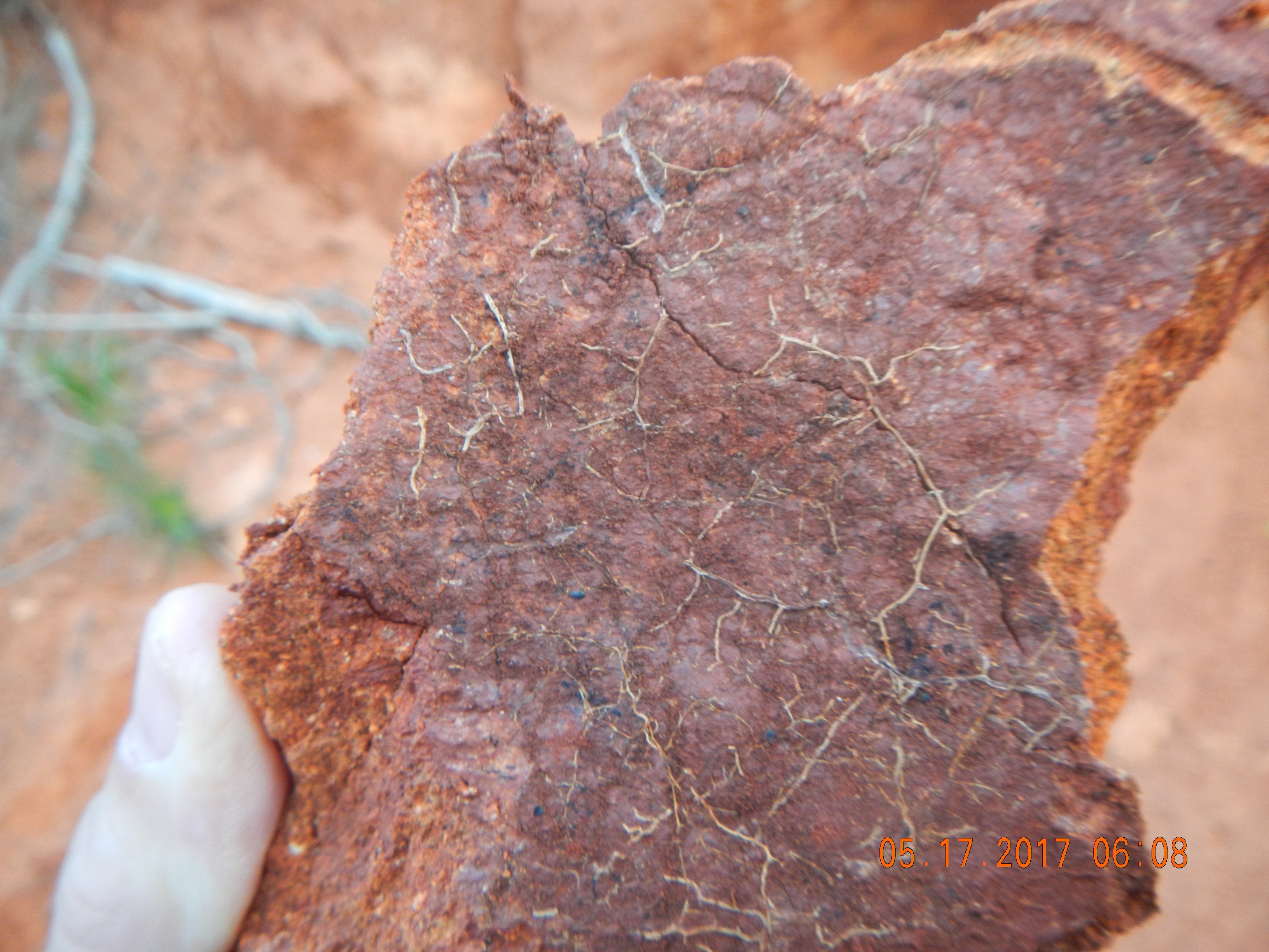
Epikarst is defined as the uppermost zone of dissolution in karst, including whatever soil cover exists. The purpose of this analysis is to explore some of the interactions among geological controls, weathering, biota, moisture flux and soil accumulation in the regolith or critical zone of karst systems.

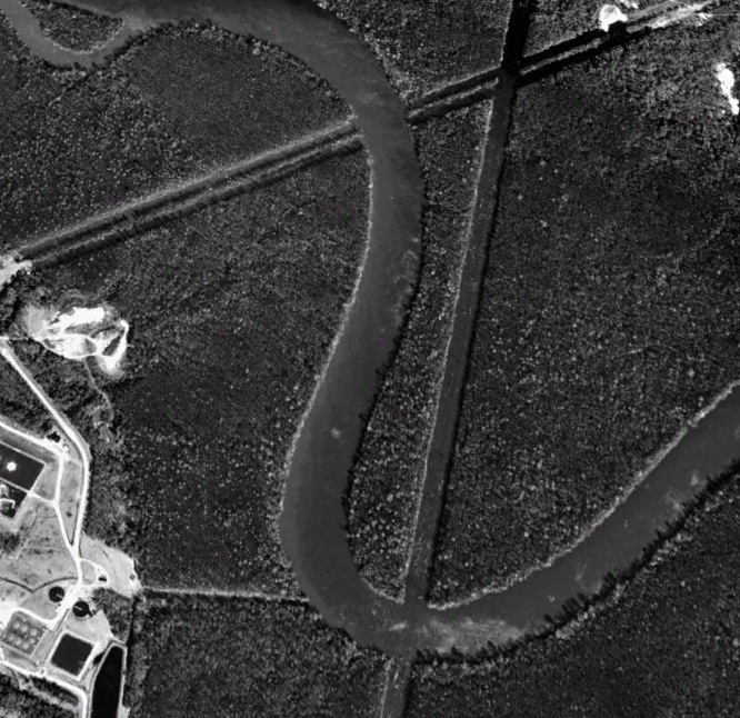
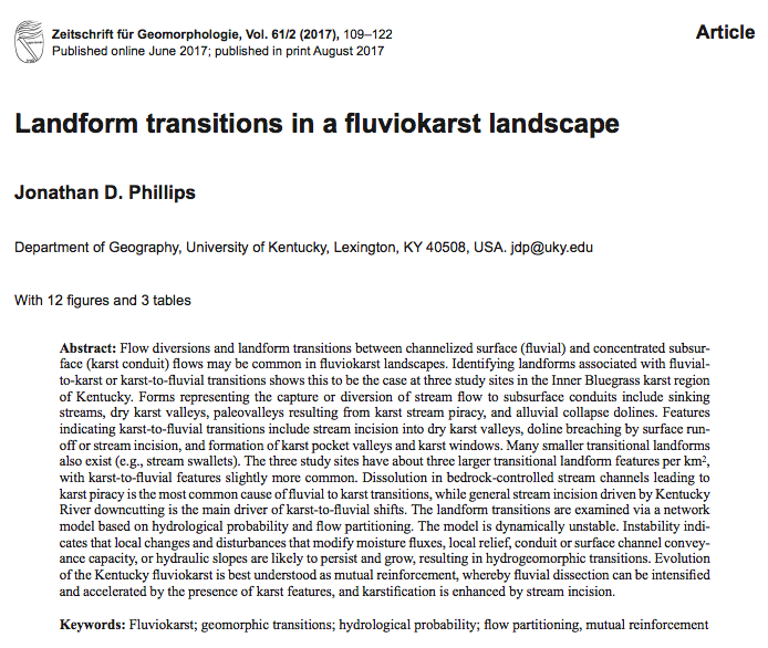
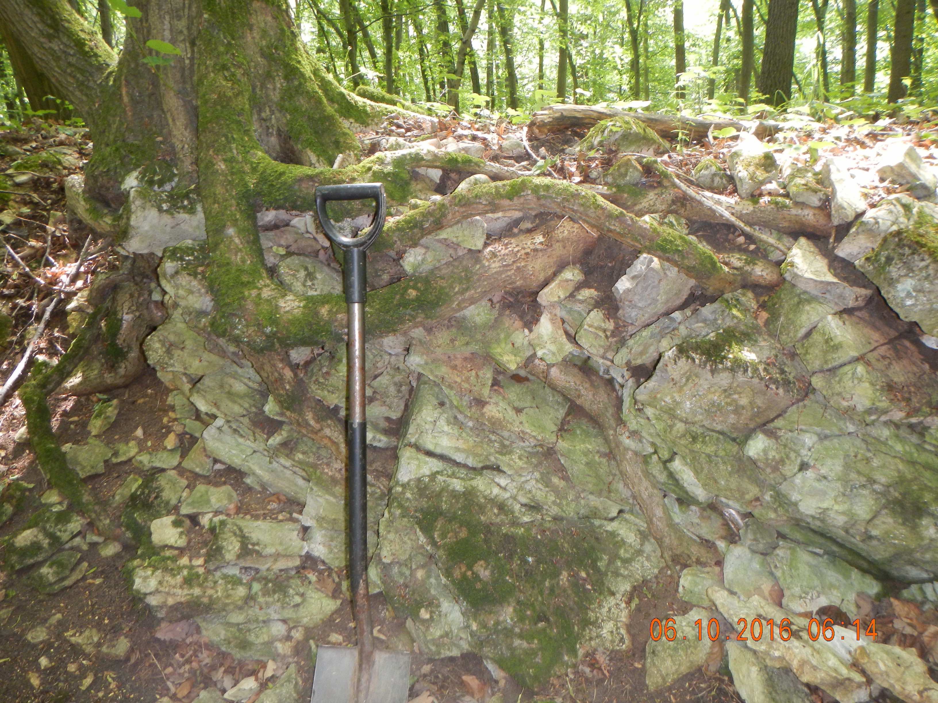
Epikarst exposed by gullying, Bowman's Bend, Kentucky

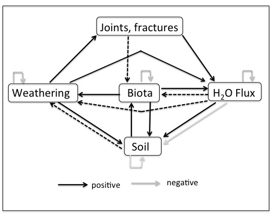
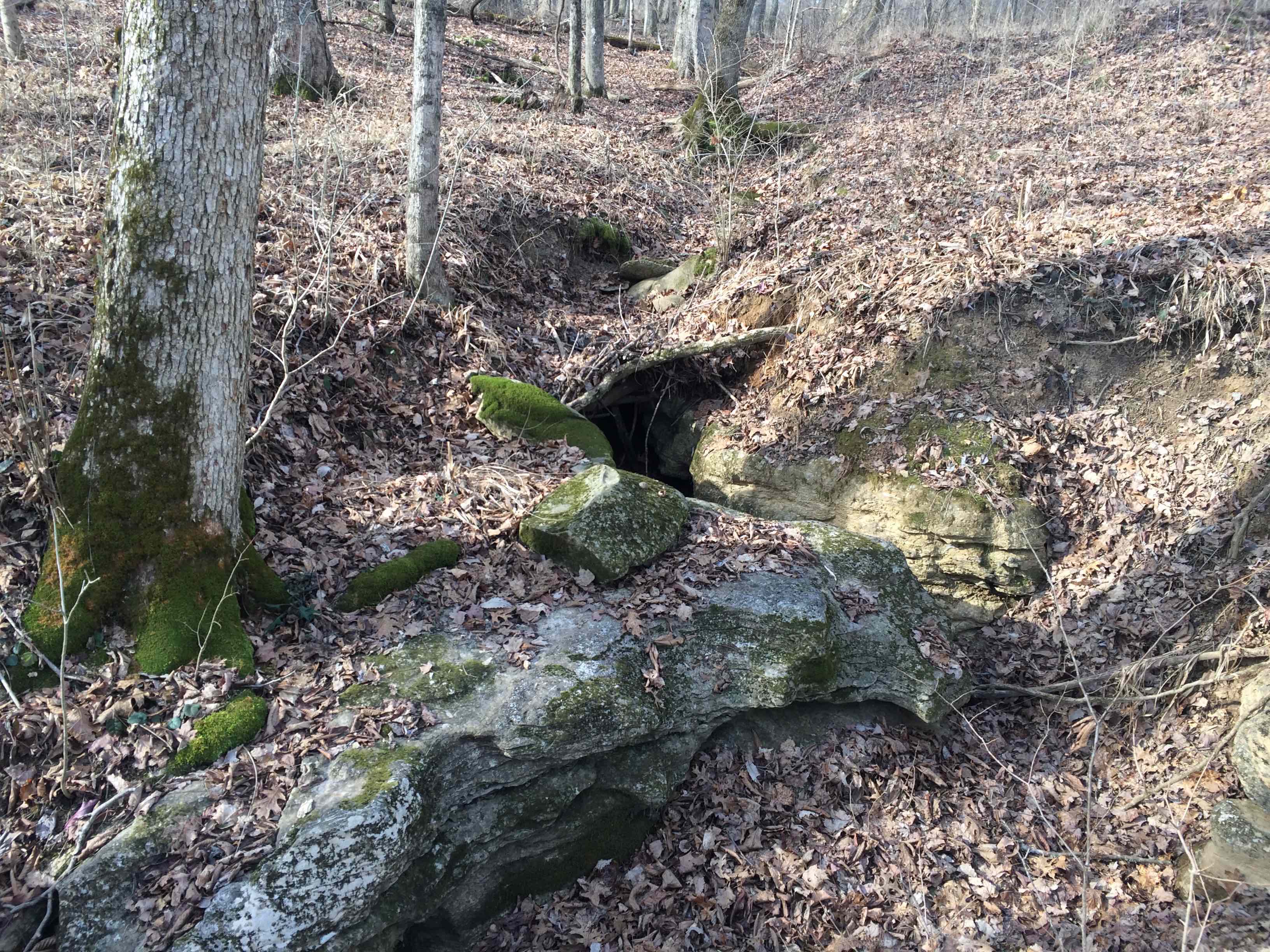
Figure 1 shows the interactions among geological controls (joints, fractures, bedding planes), weathering, subsurface biological activity, moisture flux, and soil accumulation the earlier stages of soil development in epikarst. The system is dominated by positive feedbacks because in early stages of epikarst development there is limited space for biological activity (e.g., roots), and moisture fluxes are limited by the size of joints, fractures, and incipient conduits. The other positive feedbacks reflect well established relationships among chemical weathering, enlargement of joints, etc., water availability, and organisms. I assume some external (to the system shown) limitations on biological activity and moisture flux.

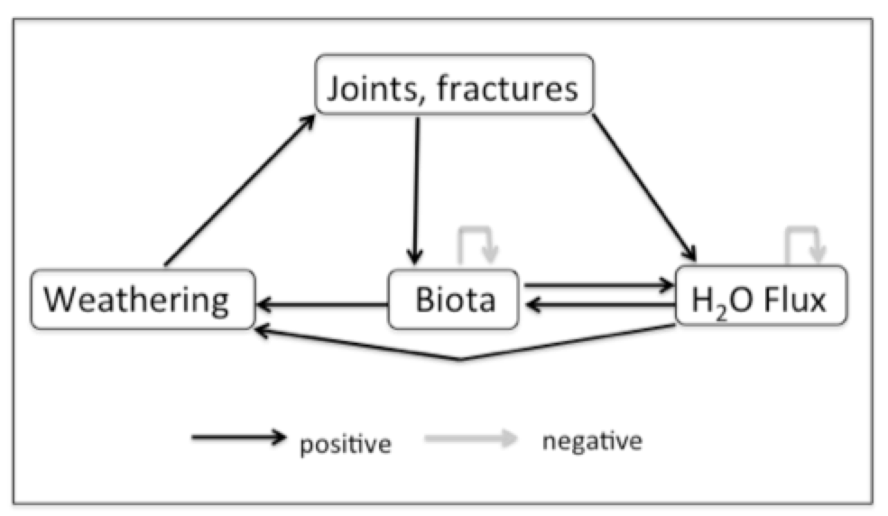
Figure 1. Interactions among structural features (joints and fractures as indicated but also bedding planes and other partings), moisture flow and penetration, biological activity, and weathering (dissolution) in carbonate rocks. These apply in situations where both biota and weathering are moisture-limited, and biota (especially roots) are limited by subsurface accommodation space. Feedback links are summarized in Table 1.

The system shown in Figure 1 is dynamically unstable. Changes such as, e.g., initial establishment of woody plants, will show persistent and disproportionately large alternations in the system state. In the example of roots, their growth accelerates water flux into and within the subsurface (via stem and rootflow, root suction, and promotion of infiltration, which in turn facilitates root growth). Both of these factors enhance weathering, which provides more access for moisture and space for roots. This instability thus promotes continued, and sometimes accelerated, development of epikarst and root zones.

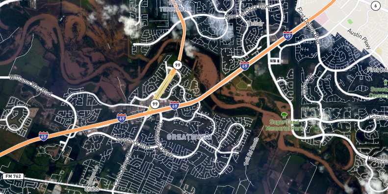
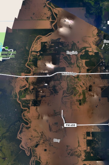
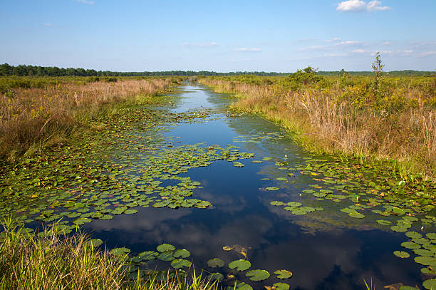
Recently exposed limestone, south central Texas. 

The weathering and biological activity also promote development of a soil cover, which is added to the system in Figure 2. Weathering, biotic activity, and subsurface moisture all promote soil development, which in turn improves edaphic conditions for biota and in may cases also promotes weathering, particularly in early stages. Rock weathering may be reduced under thick soil covers, but this is often less relevant in developing epikarst, where the thickest soils occur in widened vertical joints.  However, some of the key feedback relationships weaken or become inactive in more advanced stages of epikarst development. In particular, subsurface biotic accommodation space for roots may no longer be a limiting factor, and both weathering and biotic activity may become limited by factors other than moisture supply.

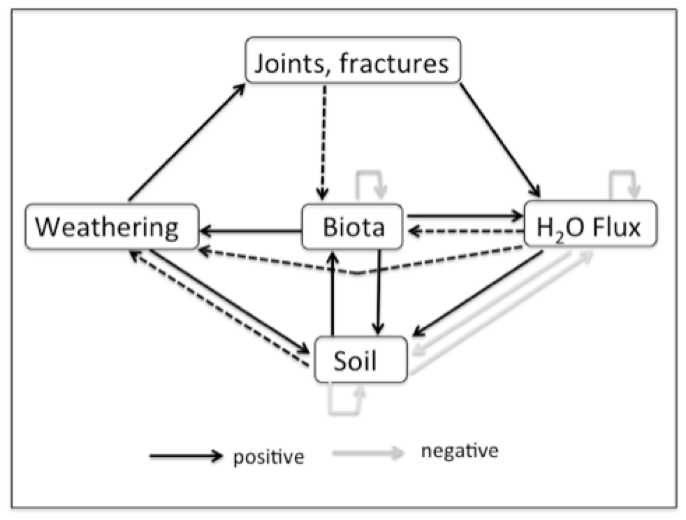
Figure 2.  Interaction system with soil added (see Table 1 for explanation). Soil component includes soil development as a surface layer and/or accumulation in joints. Dotted lines indicate links that are positive when present, but that may become inapplicable as epikarst and soil development proceeds.

The system shown in Figure 2 is dynamically unstable when the feedbacks shown as dotted lines are present. However, when they are removed the epikarst system becomes dynamically stable and resilient to small changes or disturbances, implying much more slowly changing conditions.This model suggests that plants (particularly woody plants and trees, which are most likely to have roots in contact with bedrock) are effective ecosystem engineers in epikarst. They help create the dynamically unstable conditions during which belowground biological accommodation space and moisture availability tend to steadily increase, up to the point that subsurface space and water are no longer chronic limiting factors for organisms.

When exposed rock or thin soil epikarst is colonized by plants, ecological filtering and selection presumably favor plants better able to exploit bedrock joints, fractures, and bedding planes. However, the overall enhancement of the epikarst and regolith for biota in general is an emergent outcome of the network of biogeomorphic and ecohydrological interactions.

Table 1. Brief explanation of feedback links in Figures 1-2.

¹Within table, “joints” indicates joints, fractures, bedding planes in general.

Stability analysis--details

The systems shown in Figure 1 and 2 dynamically unstable by the Routh-Hurwitz criteria (see Phillips, 1992; 1999 for explanation in a geomorphology/pedology context and Puccia and Levins, 1985; Cesari, 1971 for a mathematical treatment). However, the system becomes dynamically stable if the dotted-line links shown in Figure 2 are removed. This implies unstable self-reinforcing growth or acceleration of weathering, joint space or size, moisture flux, and biological activity as long as biota are limited (or, looked at another way, stimulated by additional) subsurface accommodation space and moisture supply, and weathering is moisture (rather than reaction) limited. Technically (mathematically) the instability would apply also to reductions in any component, but since weathering and its effects are irreversible, the growth situation is most relevant here.

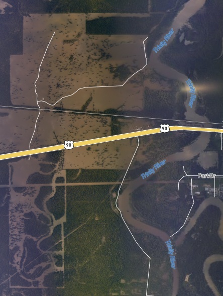
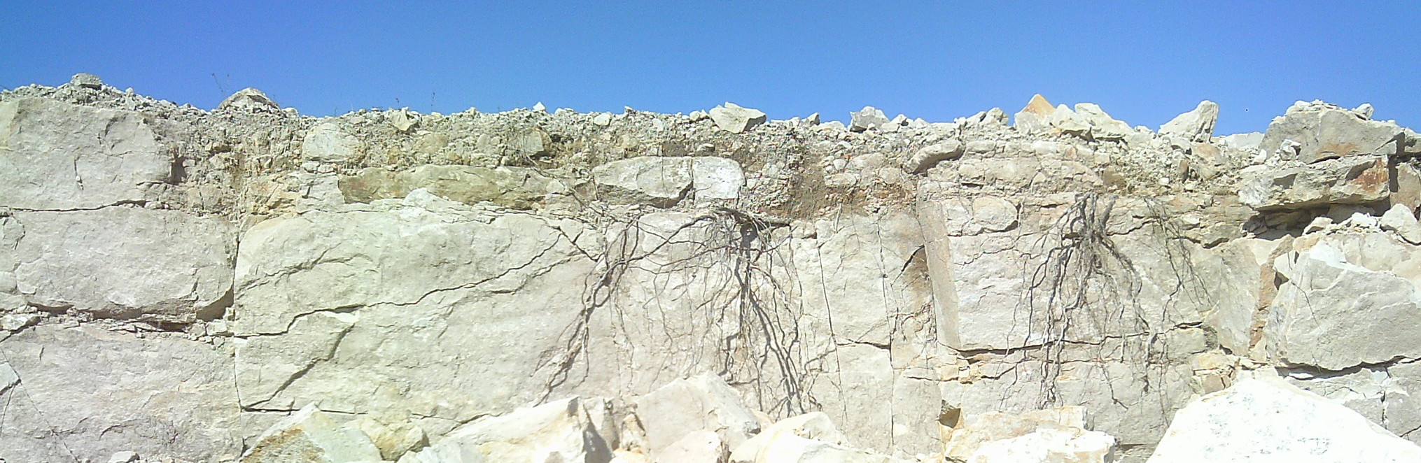
Root-rock interaction, Bohemian karst, Czech Republic. 

Including soil does not change the general outcome of the stability analysis, but puts more emphasis on the system reaching a stage where moisture flux, biotic activity and soil development become self limiting (or externally limited). The analysis of this configuration also suggests that plugging of voids with sediment due to water flow tends to enhance the unstable growth phase, while subsurface water erosion promotes dynamical stability.

Table 2 shows the interaction matrix, with links that appear as dotted lines in Figure 2 highlighted. Table 3 shows feedback at level i (F_i) for the without soil (N = 4) and with soil (N = 5) cases. The first Routh-Hurwitz criterion for stability is that all F_i < 0. In Table 4 these equations are interpreted with respect to this criterion.

.Table 2. Interaction matrix for Figures 1-3. Links that appear as dotted lines in Figures 2 and 3 highlighted.

Table 3. Feedback at level i (F_i) for the four-component (without soil, Figures 1, 2) and five-component (including soil, Figure 3) model configurations. See Puccia & Levins (1985) for calculation methods. Links that appear as dotted lines in Figure 2 highlighted.

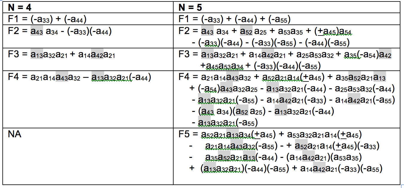
Table 4. Conditions for possible stability (F_i < 0) for Table 3.

Key differences relative to non-carbonate systems

Many of the feedbacks and interactions described above could be relevant to any, or many, critical-zone or regolith situations. However, some key potential differences associated with non-karst, non-carbonate settings are shown below (Table 5). The models above are based on an assumption of carbonate rock with only minor amounts of insoluble material, and of sufficient thickness to accommodate full development of the root zone.

Table 5. Potential key differences, carbonate vs. non-carbonate settings.

Key questions

•The concept of moisture-limited vs. reaction-limited weathering is well establishing in the literature on development and enlargement of karst fissures and conduits. There is o reason to expect that the phenomenon does not occur in epikarst development as well--is there?

•Does vegetation indeed become less water limited as epikarst evolves?

•What is the relationship between soil thickness and weathering rate in epikarst? Does the "humped" soil production function apply?  Exposed limestone weathers quite readily without any soil sover, and the irregular, discontinuous geometry of the weathering from and concentration of soil in enlarged joints may obviate or obscure any relationship between soil thickness and rock weathering rates, as water and biota are rarely far removed from rock.

•What is the role of subsurface moisture flow in depositing vs. eroding soil and sediment?

Finally, the key question is whether there exists detectable threshold or mode switch from unstable rapid growth of epikarst driven by ecosystem engineer effects of tree roots, to stable steady-state or slow growth.

The bottom line

I am confident that the interactions among rock weathering, moisture flux, biotic activity (especially roots), and soil/regolith development operate such that plants function as ecosystem engineers (EE) to produce conditions increasingly suitable for woody vegetation, up until the point that factors other than moisture and rooting space become limiting. I am also confident in the fundamental dynamical instabilities that underlie the phenomenon.

As the questions above indicate, I am less confident that I have all the details correct, and how and whether the stable condition occurs. I am moderately confident that the ecosystem engineering is non-specific--that is, the process creates generally better conditions for any woody plants and vegetation in general suited to the habitat, rather than the engineer species specifically. To the extent that they are self-replacing this is likely due to the availability of propagules rather than the EE effects. That is if, say, a chinquapin oak facilitates weathering and soil formation and improves plant habitat (and here in central Kentucky, they do) and another of the same tree replaces it, this is because there are plenty of chinquapin acorns around, not because the soil and epikarst has been made chinquapin-friendly relative to other species.

The biogeomorphic EE discussed here is contingent and emergent: Contingent on an epikarst environment (I have written on contingent biogeomorphic EE in karst here). Emergent in the sense that it derives from the particular biogeomorphic interactions in epikarst rather than being inherent in the extended phenotype of the EE organisms.

References

Cesari, L., 1971, Asymptotic Behavior and Stability Problems in Ordinary Differential Equations: New York, Springer-Verlag, 271 p.

Phillips, J.D. 1992. Qualitative chaos in geomorphic systems, with an example from wetland response to sea level rise. Journal of Geology 100: 365-374.

Phillips, J.D. 1999. Earth Surface Systems. Complexity, Order, and Scale. Oxford, UK: Basil Blackwell.

Puccia, C.J., Levins, R., 1985. Qualitative Modeling of Complex Systems. Harvard University Press, Cambridge, MA.

(posted 22 September 2017)

Geomorphology has just published a special issue on anthropic sedimentation in fluvial systems, in the centennial year following the publication of G.K. Gilbert's seminal Hydraulic Mining Debris in the Sierra Nevada. L. Allan James (AJ) edited the special issue, along with Scott Lecce and myself. Lots of good stuff in there, if I do say so myself. The issue includes an article coauthored by AJ, Scott and myself, titlled A centennial tribute to G.K. Gilbert's Hydraulic Mining Débris in the Sierra Nevada. The abstract is below, and you can download it here:

While Scott and I did enough work to deserve having our names on this, AJ really deserves most of the credit. He conceived the whole enterprise, recruited us to help, and was truly the lead author on the article above and the short introduction to the special volume. 

                                                                                                       G.K. Gilbert

Fluvial geomorphology fans celebrated publication of the special issue by donning Gilbert-type beards, following the lead of Houston Astros pitcher Dallas Keuchel, who idolizes Gilbert. 

Years ago, in my days at East Carolina University, M.A. student Don Belk (now a planner with the N.C. Department of Commerce) and I worked on issues related to hydrological restoration of artificially drained wetlands in eastern North Carolina. Basically, we found that something closely approaching the pre-drainage hydrology could be achieved in most cases by simply not maintaining the drainage ditches and canals (see this, that, and the other). In this flat, wet topography and humid subtropical climate the anthropic channels quickly accumulate sediment, organic debris, and living vegetation, losing their conveyance capacity and essentially becoming linear detention ponds in a few years. Thus, except for some local water table drawdown during dry spells in the vicinity of the ditches and canals, and whatever peat may have oxidized when the artificial drainage was working, the hydrology can be passively restored. If you don't believe me, ask someone who farms artificially-drained land in the N.C. coastal plain--they'll tell you they have to clean out the ditches every two to five years.

Poorly maintained drainage canal in the Croatan National Forest, N.C. In this case poorly maintained is a good thing!

Later on (Don & I were doing our thing about 30 years ago) others added a lot more detail on the processes and mechanisms involved in the loss of conveyance in the artificial channels, including some of my friends and successors at ECU (see, e.g., this).

What we recommended based on our work three decades ago would fall into the category of what is now called passive restoration. In the case of the wetlands we were studying, all you really needed to do was stop maintaining the drainage infrastructure. You do not need to fill in the canals, haul in new substrates, do any landscaping, or bring in nursery plants (unless the propagule source for the desired species has been eliminated). Passive river restoration seems to be at least superficially similar, as it is based on letting fluvial and ecological processes (especially those related to floods and post-flood recovery) operate unimpeded.

I was reminded of all this by Michael Groll's just-published article in Geomorphology: The passive river restoration approach as an efficient tool to improve the hydromorphological diversity of rivers – Case study from two river restoration projects in the German lower mountain range. The European Water Frame Directive favors passive river restoration for its low cost and reliance on natural processes. Groll's study tested its efficacy. The abstract is below:

Basically, Groll found that passive restoration can work pretty well--except not so much in impounded sections. That not only points to the importance of at least semi-natural flows, but also to a key difference between this case and those N.C. wetlands. In any kind of restoration project, you have to quit doing whatever it was that degraded the system to start with. In some cases--drainage canals in eastern N.C.--you can just stop maintaining them and they relatively quickly lose the capability to modify the hydrology. You don't have to fill them in. In the case of impounded sections of river, you need the relatively unimpeded flows and therefore the dam has to go. You generally can't just let it deteriorate naturally, because that usually takes too long and may pose serious hazards.

Overall, however, my read of the paper is that it supports the potential for passive river restoration (PRR), at least where flow is not impounded. However, implementing PRR requires overcoming some conceptual and perceptual obstacles:

•Stream restoration and rehabilitation is too often based on a narrow and fundamentally misguided view that there is some (single) "right" or "natural" state for a stream to be in. This ignores the natural variability of geomorphic and ecological systems in general, and streams in particular. It is also often based on normative steady-state or "balance of nature" notions that (however useful they may be as baselines, benchmarks, or simplifying assumptions in models) do not accurately reflect the real world.  In this view PRR that does not seem to be leading toward the putative normative state would be viewed as a failure even though it might be working just fine. Previous blog comments on these issues are here.

•PRR requires a range of flows; particularly high flows. This necessitates a view of floods as necessary and desirable occurrences rather than as hazards to be controlled.

•Change ≠ degradation. Fluvial systems undergo changes large and small, some of them partly or mostly attributable to unintended human impacts. When such changes are readily observed, they are often accompanied by a well-meaning desire to "put it back like it was." But sometimes the change is not necessarily harmful, even if triggered by human activity.

•PRR in some cases amounts to doing little or nothing, and politicians and managers are sometimes under pressure to do something. There are also contractors and consultants with vested interests in river engineering and more active restoration.

The time is right to aggressively pursue passive restoration. Other than eliminating the activities that degraded the system, consider the option of doing nothing.

(posted 19 September 2017)

As I write, the lower Brazos River west of Houston, Texas, has been in flood for more than seven days, and is likely to remain that way another week, minimum. The peak five days ago occur occurred at a gage height of 52.65 feet at the Rosharon gaging station (third highest ever, going back more than a century), and is still only about four inches below that, and not dropping appreciably. At the next gaging station upstream, at Richmond, TX, the stage was the highest on record. On August 31, near the peak at Rosharon and with water levels still above the designated major flood stage, U.S. Geological Survey personnel went to the site and measured the flow.

Location of the Brazos River Rosharon gaging site.

We've heard a lot about the various individuals and organizations doing the brave, difficult work associated with rescues after tropical storm Harvey unleashed 1000 to 1300 mm (40 to 50 inches) of rain on the Houston area. At first, getting out to collect some hydrological data, while commendable, may sound less important. But monitoring streamflows, forecasting floods, and issuing warnings that can save lives and property depends on these river gaging stations. The continuous monitoring of discharge is based on stage-discharge relationships, correlating water levels with flow rates. And, particularly in alluvial rivers such as the lower Brazos, these relationships change over time as the river channel naturally varies. Establishing, maintaining and updating the stage-discharge curves requires that somebody--usually USGS personnel--go into the field about a dozen times a year to measure velocities, widths, and depths. It is important to get these measurements across a range of flow conditions, including floods.

Fieldwork during a flood is at best difficult, and can be dangerous. Having done it myself during several floods much smaller than this one, I admire and appreciate this work. The August 31 set of measurements at the Rosharon site (not the only ones USGS did in the region near peak flows) are particularly interesting as well as important.

August 31 aerial photograph of the Brazos River valley near Rosharon Texas, from NOAA/USGS storm assessment (https://storms.ngs.noaa.gov/storms/harvey/index.html) 

To capture the flow headed down the Brazos valley, they had to make 12 separate "channel" measurements. Channel is in quotation marks because in addition to the main channel and a couple of sub-channels the crew measured several overflow areas of subchannels, culverts, and flooded road and field areas (you can access the data here). They self-rated the measurements as "poor" because of the difficult conditions (among other things, there is a notation of "debris heavy"), but it's the best we've got.

Only about 68 percent of the total flow of 3,372 cms (119,000 cfs) passed through the main channel. The proportion flowing through other pathways varied from less than 1 percent in several cases to >14 percent. The width of the measured sections ranged from culverts 2 to 5 m wide to the main channel at 204 m to a section of floodplain 3627 m wide. Accordingly width/depth ratios were also quite variable, from <5 in the culverts to 30 in the main channel, to >2500 on the unchannelled floodplain. The highest velocities (> 2 /sec) were at the culvert sites, and 1.65 m/sec in the main channel. The slowest were at the sheet-flow-like floodplain sections, some of which were <0.1 m/sec.

If you solve the Darcy-Weisbach equation for f, the friction factor, you get f = f(1/V²). Using 1/V² as a crude relative roughness index, roughness varied over four orders of magnitude. As you'd expect, it was lowest in the channels and culverts and highest in the unchannelled sections.

These results remind us that our binary of in-channel vs. floodplain (overbank or out-of-channel) flow masks a great deal of variability.  Many valley bottoms are quite heterogenous even without human agency, and our activities may both accelerate and impede downvalley flow, both inadvertently and purposefully.

Some other notes from this event:

•In a study of key discharge thresholds on the Brazos, I estimated a discharge of about 1000 cms as the threshold of channel instability at Rosharon. This was clearly exceeded, and occurs well below the overbank flood discharge of 1546 cms. Here I mean mechanical instability, involving potential bed, bar, and bank erosion.

•Measuring or estimating the key parameters of geomorphic change, stream power and shear stress, requires the inclusion of energy grade slope, which is not included as part of normal field measurements by USGS or anybody else. In the study referred to above I estimated S based on channel slopes and on station-to-station water surface slopes during specific events. However, these methods (while commonly used) are not very precise, and undoubtedly mask a great deal of variability. This is, in my view, the major weakness in our analyses.

•If you look at a map of the lower Brazos and adjacent Colorado River watersheds, you will notice that both are unusually and unexpectedly narrow in the lower part. This is because both have experienced watershed fragmentation avulsions. These occur when an abandoned main channel maintains an independent path to base level (in this case the Gulf of Mexico), but not as a distributary channel or anabranch. Rather, the hydraulic connection with the new main channel is lost, creating a new watershed. About 1.5 Ka, the Brazos avulsed to its current path near San Felipe, TX, upstream of Richmond. There is no regular flow from the Brazos to the old channel, now designated Oyster Creek (Bessie's Creek in the upper reaches). However, at some high flood flows--the 2017 Harvey ones, for example--water moves across the Brazos floodplain into the Oyster Creek system. About 13 percent of the August 31 flow was being transported by Oyster Creek or its overflow.  

August 31 aerial photograph of the Brazos River valley near Richmond & Rosenberg Texas, from NOAA/USGS storm assessment (https://storms.ngs.noaa.gov/storms/harvey/index.html)  

Posted 4 September 2017 

Did you ever wish you had a collection of these blog posts, all semi-organized in one quasi-coherent document? No? Well, you can get one anyway. My posts from the very first in May, 2014 up through June, 2017 have been collected in a single volume, called The Perfect Planet, now available here.

Wooooooo!!! At last!

There is, however, good news and bad news.

Good news: It is a rich compendium of my interpretations, speculations, and scientific opinions over a three-year period.

Bad news: How egotistical and self-important do you have to be to think anyone would want such a thing?

Good news: In The Perfect Planet you get JDP unfiltered by nit-picky grammar monkeys and uncensored by the scientific establishment.

Bad news: That’s because the “book” is self-produced, with no peer review and no professional copy-editing or production.

Good news: It is absolutely free (though in the form of a reduced-resolution compressed pdf file)!

Bad news: It might well be worth exactly what you pay for it.

The Perfect Place is published by Copperhead Road Geosciences, my consulting firm that is currently inactive. It is not copyrighted, and has no ISBN. It is available for download from Researchgate.

The latest issue of Earth-Science Reviews contains a couple of articles where the issue of scale linkage is front and center.  Ma et al. (2017) review the past five years or so of research on hydropedology, focusing on soil-water interactions across spatiotemporal scales.  Walker et al. (2017) outline scale-dependent perspectives on geomorphic evolution of beach and dune systems, based largely on years of collaborative work on Prince Edward Island (Canada).

Beach and frontal dune at Prince Edward Island National Park (http://www.parkscanada.gc.ca/pei)

Both papers deal with a classic, hoary problem in the geosciences—but a problem that still has not been fully solved, and that vexes researchers regularly. Soil, hydrologic, geomorphic, ecological, and climate systems are all intertwined, and all are influenced by processes ranging from molecular to planetary, and operating over time scales from instantaneous to eons.  In some senses these processes and controls as they apply to a given Earth surface system (ESS) are connected and related. However, in practical terms the details of geochemical kinetics or wind stress on a sand grain do not apply to the geological evolution of landscapes; nor do paleogeography, plate tectonics, and evolution of the atmosphere explain the response of a soil or sand dune to a storm. At the far end of the ranges, intuition and common sense alone is sufficient to justify some exclusions. For example, no one expects Walker and company to address geological evolution of the Canadian continental margin in their geomorphological studies of Prince Edward Island; no one would demand that Ma et al. place their work in a palaeopedological context. Likewise, in my study of fluviokarst landscape evolution, no reviewer insisted that I address the partial pressures of dissolved carbon dioxide. Of course, there’s a lot of room between the extremes of geological time and the time spans of fluid flows and chemical reactions. 

More than half a century ago Schumm and Lichty (1965) produced a classic statement pointing out that whether variables are dependent or independent depends on temporal scale, using examples from geomorphology. The intuitive truth of this can be formally demonstrated. For example, for an Earth surface system characterized as a set of interacting components that operate at fundamentally different scales, it has been proved that the dynamics at different scales are independent in terms of their influences on system dynamics (Schaffer, 1981; Phillips 1986; 1988).  Walker et al. (2017) embed their work in Schumm and Lichty’s framework, and extend scale considerations by providing a detailed example of “scale-aware” (their term) conceptual and functional integration of plot and landscape scales.

The dynamical stability or instability of weathering systems varies with spatial scale (Figure 6 from Phillips, 2005).

Ma et al. (2017) explicitly promote a hierarchical framework for spatial scale bridging in hydropedology. They maintain that soil physicists and hydrologists have generally viewed the relevant processes as a continuum, though I would argue that an implicit hierarchy has long existed in field-based hydrological studies.

Scale hierarchy in hydrology I proposed in 1999 (Figure 8.1 from Phillips, 1999). Each level includes the cumulative effects of lower levels and new considerations.

The hierarchical approach both Ma et al. (2017) and Walker et al. (2017) promote and illustrate is a sound one, involving linking or bridging between adjacent levels of a scale hierarchy. One formal approach is hierarchy theory, one formal expression of which is:

(Excerpt from Phillips, 2016, p. 67).

If the key components of the system are represented as a mathematical graph or network at hierarchical scale levels, it can be shown that as the number of levels increases (that is, consideration is extended up or down the scale hierarchy to broader spatial and longer temporal scales or finer spatial and shorter temporal scales) complexity increases, but at a less than linear rate. However, inferential synchronization (the ability to infer dynamics at one level from those at another) deteriorates rapidly, at a greater than linear rate. This is the phenomenon of scale decay, directly analogous to the geographical concept of distance decay (near things are more closely related than far things). For example, using the algebraic graph theory metrics of spectral radius (and closely related graph entropy) to measure complexity, and algebraic connectivity as a measure of inferential synchronization, we inevitably find something like the trends below. These are for specific examples from pedology (top) and fluviokarst flow patterns (bottom), but similar trends are found in various archetypal hierarchical graph structures.

Figures 5 and 7 from Phillips, 2016.

A set of components operating at a given scale can be considered a subgraph or subnetwork of the larger ESS. The eigenvalues (lambda) of the subgraph a are related to those of the larger system by

The unindexed lambdas are the eigenvalues of the larger system, and index d signifies a subgraph consisting of those components not included in a. The eigenvalues (the graph spectrum) describe its dynamics, and this relationship shows that the subgraphs at different scales are independent.

When common sense, intuition, empirical evidence, and formal theory all converge to the same conclusion, I think it is safe to conclude that the conclusion is sound. Scale linkage is important, but a single representation or transfer across a broad range of scales will not work. Rather, a transfer one level at a time up or down a scale hierarchy is the way to go.

References:

Ma Y, and 3 others. 2017. Hydropedology: Interactions between pedologic and hydrologic processes across spatiotemporal scales. Earth-Science Reviews 171: 181-195.

Phillips JD. 1986. Sediment storage, sediment yield, and time scales in landscape denudation studies. Geographical Analysis 18: 161-167.

Phillips JD. 1988. The role of spatial scale in geomorphic systems. Geographical Analysis 20: 359-368.

Phillips, J.D. 1999. Earth Surface Systems. Complexity, Order, and Scale. Oxford, UK: Basil Blackwell.

Phillips JD. 2005.  Weathering instability and landscape evolution. Geomorphology 67: 255-272.

Phillips JD. 2016. Vanishing point: scale independence in geomorphic hierarchies. Geomorphology 266: 66-74.

Schaffer WM. 1981. Ecological abstraction: the consequences of reduced dimensionality in ecological models. Ecological Monographs 5: 383–401.

Schumm SA, Lichty RW. 1965. Time, space, and causality in geomorphology. American Journal of Science 263: 110-119.

Walker IJ, and 6 others. 2017. Scale-dependent perspectives on the geomorphology and evolution of beach-dune systems. Earth-Science Reviews 171: 220-253.

Posted 12 August 2017

The article below was just published in Zeitchrift fur Geomorphologie. A full-text preprint version is available here. The link to the journal is here. 

Posted 8 August 2017