More than one scholarly observer has remarked in the contrast between physics, characterized mostly by deterministic, hard-and-fast laws that operate the same way everywhere and always (at least the Newtonian physics that apply to Earth sciences) and biology. Biology is portrayed as being much more fluid and dynamic, in the sense that chance (e.g., mutations) and environmental adaptations play a major role. As Gregory Chaitin (2012; a mathematician, by the way, not a biologist) puts it, biota and evolution are creative, while physics is not. This tension is sometimes portrayed or exemplified as a Newtonian (as in Isaac Newton) vs. Darwinian (i.e., Charles Darwinian) outlook. 

I have much love for both Newton (left) and Darwin, but have chosen to follow Darwin with respect to my hairstyle. 

Of course, landscapes and environmental systems are strongly and profoundly influenced by biota, and also by chance and variability. Thus, even in hydrology, a field traditionally dominated by Newtonian physics/engineering perspectives, there have been numerous calls to develop a "Darwinian" hydrology or to integrate Darwinian and Newtonian approaches (e.g.,  Harman and Troch, 2014). Among other things, these proposals focus on the value of the Darwinian foci on variability, history, and multiple possible evolutionary pathways--All drums I have beat repeatedly over the years. 

I am a strong proponent of the biotic role in Earth systems and the strong coupling and reciprocal interactions between biotic and abiotic phenomena. I also recognize the value of organic metaphors for understanding and explaining landscapes. However, I have always stopped short of viewing or presenting Earth surface systems as superorganisms or claiming that Darwinian natural selection applies directly to geosciences (though selection phenomena more generally are certainly applicable; see this post). 

While I agree that the biota that live in and help shape landscapes are creative, can we legitimately argue that landscapes and Earth systems, as entities in and of themselves, are?  That's what I will be exploring in (hopefully near) future posts.

Reciprocal interactions occur among biota, soils, and landforms, along with coevolution. But is there creativity at the scale of landscapes and Earth surface systems? (Stump hole in the Piedmont/Sandhills transition zone, Moore County, North Carolina)

-----------------------------------

Posted 2 May 2018 

Historical contingency in fluviokarst landscape evolution was just published in Geomorphology 303: 41-52.  When I first came to central Kentucky in 2000 I began noticing the strong contrasts in landscape and landform development on inner vs. outer Kentucky River incised meander bends. Investigating this and related phenomena has occupied me off and on ever since. Only a few years ago I realized that given the nature of bend development over the past 1.5 Ma or so, the bend interiors represent a chronosequence of landforms. This paper exploits those chronosequences, using graph theory, to explore the role of historical contingency.

Chronosequence of strath terraces (T1, T2, T3) and other geomorphic surfaces at Polly’s Bend, Kentucky. The surfaces nearest the river are youngest; those farther away are oldest.

Chronosequence of strath terraces (T1, T2, T3) and other geomorphic surfaces at Bowman’s Bend, Kentucky. The surfaces nearest the river are youngest; those farther away are oldest.

Reference: Phillips, J.D., 2018. Historical contingency in fluviokarst landscape evolution. Geomorphology 303: 41-52.

Previous blog posts on related topics: 

Evolution of Polly's Bend: Initial conditions, bend extension

Karstification of Bowman's Bend

Landform transitions in a fluviokarst landscape

Posted 5 February 2018

Below is a picture of raindrop impact craters after a rain last month on a beach along the Neuse River estuary, N.C. The spot pictured has no overhanging trees or anything else, so the craters represent direct raindrop impacts. As you can see, assuming crater size is related to drop size, they represent a large range (the largest craters pictured are roughly 10 cm in diameter; the craters must be at least slightly larger than the drops). Rainsplash is a significant factor in soil erosion--even if not directly important, the process is key for dislodging grains or particles that are then transported by runoff. Drop impact also influences surface crusting and sealing, and thereby hydrological response. So, I got to thinking, what is the potential significance of such a large variation in drop size?

Kinetic energy is given by KE = 0.5 m V^², where m is mass in kg, and V is velocity in m/sec. A 2 mm diameter raindrop has a mass of 4.19 mg and a terminal velocity of about 6.26 m/sec. This gives a kinetic energy of about  0.00008 joules per raindrop.

Terminal velocity depends on raindrop size, which is directly related to drop volume, as density is constant at 1 g/cc. Some formulae estimate velocities for a given raindrop event based on the median drop size (diameter), D_50, in the form

V = a D₅₀ exp(^{b D50}),

where a and b are constants, equal to 48.54 and -1.95, respectively, in the formula developed by J.O. Laws, who did seminal work on this in the 1940s.  Median drop size, in turn, is often related to rainfall intensity.

For a single raindrop terminal velocity is reached when air resistance is equal to the gravitational pull.  Raindrop mass scales as the cube of diameter, and we can assume resistance varies with surface area of the drop, which scales as the square of diameter. Thus V = f(D^^0.5).

What this all adds up to, assuming spherical drops, is that kinetic energy of raindrops varies as the fourth power of drop size: KE = k D^⁴, where k is a proportionality constant. Thus, for example, a doubling of raindrop size increases kinetic energy by a factor of 16.

The photographs above and below represent about a six-fold range of diameters, assuming drop diameter is proportional to impact crater size. This represents a nearly 1300-fold range of kinetic energies!

Raindrop impact craters, eastern North Carolina.

This in turn makes me wonder whether variation in raindrop size--and therefore kinetic energy and force--plays a role in producing local spatial variations of hydrological and soil erosion response, as in both cases dynamical instabilities tend to cause minor initial variations to be exaggerated over time. I have generally assumed that these minor initial variations are associated mainly with surface and soil properties rather than precipitation inputs, but now I wonder.

Highly variable microtopography related to soil erosion. Does raindrop size variability play a role in initiating such variability? Top: Lake Bogoria area, Kenya (World Wildlife Federation photo). Bottom: Denbe Bengul, Eritrea (Panoramio).

Posted 2 February 2018

In my experience, beer cans and bottles discarded as litter in the kinds of places where I recreate and do field work are about 80 percent Bud Light, 17 percent other undrinkable watery American light beers, and 3 percent all other brands combined. Recently, however, at a site along the Neuse River, North Carolina, the two dozen or so trash bottles I saw  on the ground included NO Bud Lights!

I am not well versed enough in contemporary cultural or economic geography to speculate as to whether this is a local anomaly, a shift in taste preferences for the kind of sh*tbag Bud Light drinkers who trash the countryside, or an expansion of litterbug behavior beyond the Lite beer crowd.

Of course, when it comes to beverage container trash, no brand of beer, soda pop, or anything else comes close to the mass or volume of plastic water bottles. Why don't you people use canteens, reusable bottles, or at least recycle these things?

Posted 22 January 2018

Ferricretes are soil or sediments cemented together by iron oxides. In eastern North Carolina, reducing conditions often prevail on the broad, flat interfluves. Under these conditions Fe is reduced, and soluble. Groundwater flow from these areas toward the major river valleys transports this dissolved ferric iron. When the groundwater discharges along the valley side slope it comes in contact with oxygen, and the iron oxidizes to its ferrous form. These iron oxides coat whatever material exists at that location--sand, clay, etc.

Limonite ferricrete at Fishers Landing, NC. The piece at the top is about 40 cm long. 

When these iron-coated materials are exposed, typically by bank or shoreline erosion, they harden into rock-like ironstones--ferricretes. Once the Fe-coated material is exposed, it can harden very rapidly; within a year or two. They are hard enough so that geologists erroneously interpreted them as sandstone layers into the 1990s. When I read about a similar ferricrete formation process in Australia, I realized that the ironstone I'd been seeing might be formed the same way; some of them were very clearly NOT sandstones.

Recently exposed (as of January 2018) unhardened Fe-coated material.

I studied these ferricretes about 20 years ago (Phillips et al., 1997; Phillips, 2000), and had an opportunity to observe the process in action recently.  Shoreline erosion along the Neuse River estuary at Fishers Landing (near New Bern, NC) has recently exposed some iron-coated material that is still unhardened. However, the entire shoreline is littered with ferricrete fragments ranging from pea gravel to small boulder size.

Ferricretes scattered along eroding shoreline, Fishers Landing.

"Ferricrete hash" derived from abrasion and wave erosion of ferricretes.

REFERENCES

Phillips, J.D., Lampe, M., King, R.T., Cedillo, M., Beachley, R., Grantham, C. 1997. Ferricrete formation in the North Carolina Coastal Plain. Zeitschrift fur Geomorphologie. 41: 67-81.

Phillips, J.D. 2000. Rapid development of ferricretes on a subtropical valley side slope. Geografiska Annaler 82A: 69-78.

Posted 19 January 2018

Just published:

Phillips, J.D., 2017. Geomorphic and hydraulic unit richness and complexity in a coastal plain river. Earth Surface Processes and Landforms 42: 2623-2629. 

The abstract is below, and a preprint version is available here. 

Posted 6 December 2017

The development and change over time (evolution) of geomorphic, soil, hydrological, and ecosystems (Earth surface systems; ESS) is often, perhaps mostly, characterized by multiple potential developmental trajectories. That is, rather than an inevitable monotonic progression toward a single stable state or climax or mature form, often there exist multiple stable states or potentially unstable outcomes, and multiple possible developmental pathways. Until late in the 20th century, basic tenets of geosciences, ecology, and pedology emphasized single-path, single-outcome conceptual models such as classical vegetation succession; development of mature, climax, or zonal soils; or attainment of steady-state or some other form of stable equilibrium. As evidence accumulated of ESS evolution with, e.g., nonequilibrium dynamics, alternative stable states, divergent evolution, and path dependency, the "headline" was the existence of > 2 potential pathways, contesting and contrasting with the single-path frameworks. Now it is appropriate to address the question of why the number of actually observed pathways is relatively small.The purpose of this post is to explore why some developmental sequences are rare vs. common; why some are non-recurring (path extinction), and some are reinforced.

Path Extinction

When considering all possible pathways that do not violate governing laws and principles, some are inherently unlikely. For instance, pathways involving infrequent, low-probability events (e.g., bolide impacts, mega-floods, volcanic super-eruptions, EF5 tornadoes) will be far less common than pathways that do not require these events. Independently of these variations in probability, this section considers why some evolutionary pathways that do occur may be non-recurring, or at least inhibited in reoccurrence. It is axiomatic that path extinction is partly dependent on time scales. Pathways driven by or associated with glacial-interglacial cycles, for instance, cannot recur over shorter time periods.

Literal Extinction

Environmental change may eliminate some necessary controls or resources of a pathway, such that it cannot reoccur. For instance, there exist types of paleosols that do not have even an approximate modern analog, because their pedogenesis was influenced by, e.g., an atmospheric composition that no longer exists, and/or by extinct biota with no modern analogs. Over shorter time scales, landscape evolution, pedogenesis, or succession patterns linked to, e.g. a glacial climate cannot recur in currently unglaciated zones until a new glaciation occurs.

Unfavorable Outcomes

Some ESS evolutionary paths may lead to outcomes or states that are suboptimal, inefficient, or dangerous for biota involved, or that are dynamically unstable, vulnerable or fragile. With respect to, e.g., animal ecology, these bad outcomes condition against future choices and behaviors that involve those paths. This may occur due to conditioning, or learning/teaching to avoid these behaviors, or because death or lack of reproductive success culls any genetic tendency toward these behaviors.

Frost flowers occur when ice is extruded from long-stemmed plants under freezing conditions when the ground is not already frozen. They are fragile and unstable. (Photo credit: greatwhitenorth.blogspot.com)

With respect to (partially or wholly) abiotic features such as landforms, soils, or hydrologic systems, if the end-state of a pathway results in instability or fragility, the state simply does not last long. Therefore, given our dependence in many cases on reconstructing pathways from historical evidence, they are less likely to be observed or preserved (e.g., in stratigraphy). This vulnerability and instability may thus result in a kind of apparent extinction, where things that do happen are simply rarely, if ever, observed.

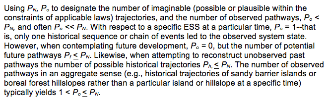
Hillslopes that develop to slopes steeper than the angle of repose eventually fail, as did this one in north Queensland, Australia. Thus the unstable steeper outcomes do not last and are not preserved.

Negative Feedbacks

The biotic phenomena mentioned above constitute negative feedbacks against certain pathways, reducing their future occurrence. These phenomena may also apply to partially abiotic ESS features, too, due to the effects of ecosystem engineering and niche construction. For example, chemical weathering feedbacks may limit runaway global cooling or warmer to global icehouse or greenhouse conditions. Landforms and soils may absorb many environmental effects of biota, thereby buffering the atmosphere, hydrosphere, and lithosphere from some biotically-induced changes. These phenomena essentially prune potential evolutionary pathways.

More generally, many evolutionary pathways in ESS are inherently externally or self-limited. Phillips (2014) gives examples for geomorphic systems involving threshold-mediated modulation, whereby exceedence of thresholds (for instance, positive or negative mass balances) may limit development on a particular trajectory.

Irreversible and Self-Limiting Phenomena

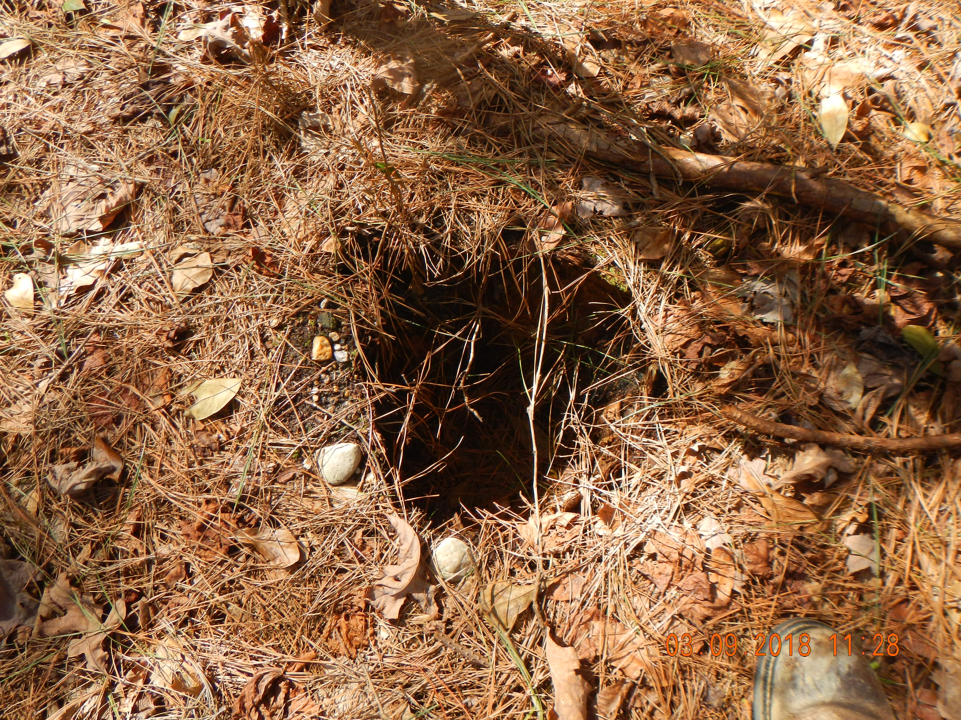
Weathering processes are often irreversible, and chemical weathering may depend on the availability of weatherable minerals. These are examples of situations where, at least over many time scales, some paths may be unrepeatable due to material limitations. A trajectory involving the weathering of a granitic rock mass, for instance, cannot be repeated (in that location). For another example, once the carbonate rock in a terrane has been consumed, pathways involving karstification are no longer possible.

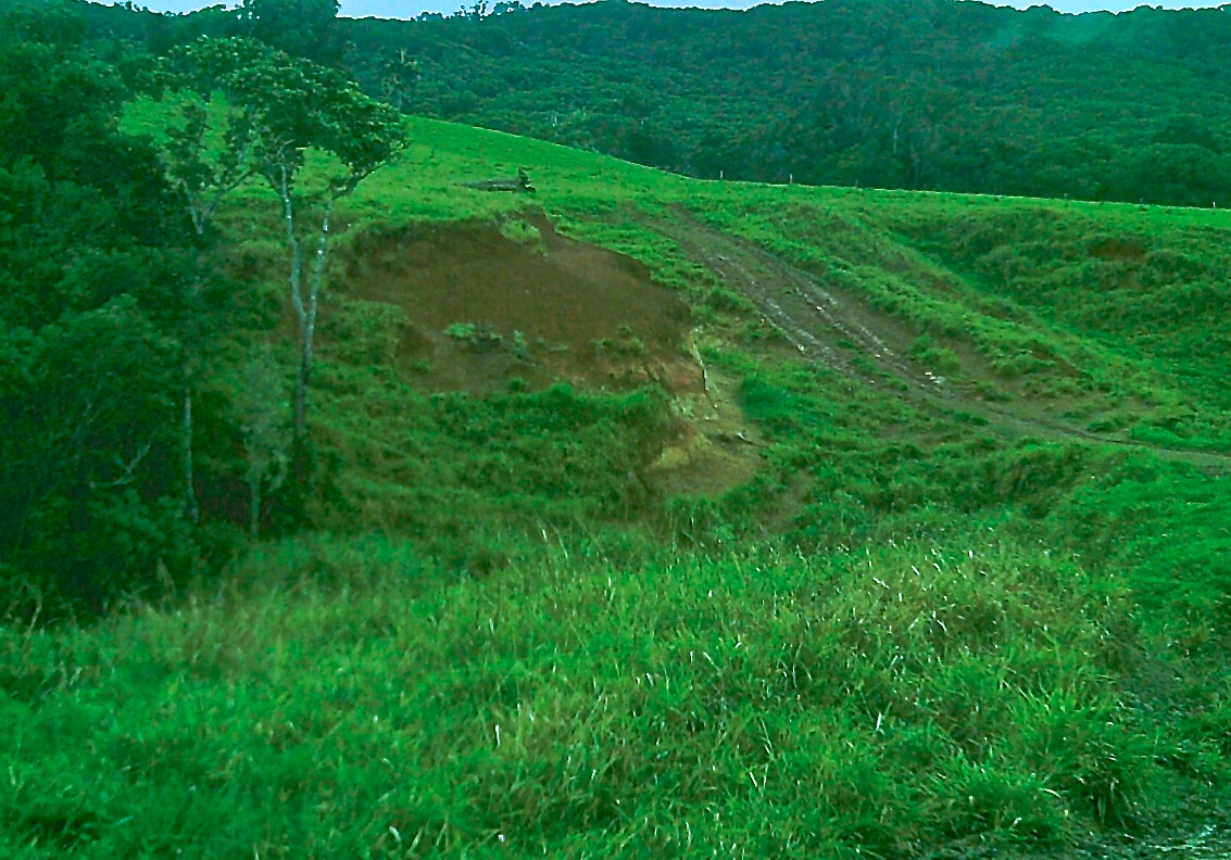
Weathering of the basalt leading to development of this Phillipines weathering profile is irreversible (photo credit: V.B. Asio).

Path Instability

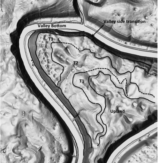
In this case instability refers to developmental sequences themselves, rather than states at the end of (or along) the sequence. Path instability means that once a developmental path is perturbed, it does not return to its pre-disturbance trajectory, but takes a new pathway. This concept is discussed here in the context of chronosequences, and examples given of soil chronosequences.

Path Reinforcement

Here we consider why and how some pathways, however probable their initial occurrence, may be enhanced or encouraged with respect to recurrences. Pathways dependent on frequent, common events are more likely to recur, other things being equal. Thus, for instance, post-fire vegetation succession patterns may be common in environments characterized by frequent fire, and post-flood recovery pathways may be recurrent in rivers that flood frequently.

Selection

The most fundamental phenomenon in path reinforcement is selection. While Darwinian natural selection strictly applies to individual organisms, selection in a broader sense applies to ESS in general, with a probabilistic tendency for development and preservation of more stable, efficient, and resistant structures and pathways. I have expounded on this in several previous posts: 1, 2, 3. Thus we can expect that evolutionary trajectories leading to these outcomes are more likely than others.

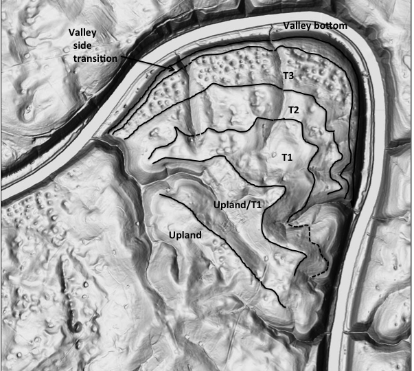
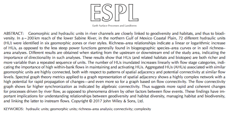
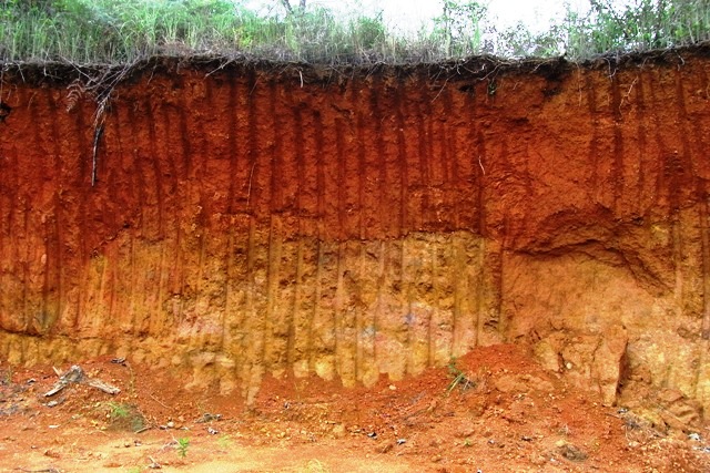
Channels are the most efficient way to move water. Thus the evolution of hydrologic systems repeatedly leads to the development of channels (Sabine River, TX/LA).

Resistance and Resilience

Pathways leading to outcomes that are resistant to change or disturbance, or resilient (able to recover) will be more often observed and preserved. Thus, independently of selection for resistance and dynamical stability, this can lead to apparent reinforcement due to more common recording.

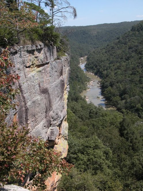
Sandstone often occurs with less resistant rock in sedimentary sequence. Due to resistance selection during erosional dissection, sandstone ridgetops are a recurring feature in areas of eroded sedimentary rock (Big South Fork National Recreation Area, Kentucky).

Path Stability

Again, this refers to stability of developmental sequences themselves, rather than system states. Some pathways are dynamically stable, and resume following perturbations. Some generic examples are given in this paper. In general, divergent radiation-type sequences are highly robust to disturbances. However, due to the nature of such pathways, while the general structure is path-stable, the specific divergent outcomes may be quite variable. Linear sequential and some convergent patterns are also somewhat robust to disturbance. Thus, where classic linear successional sequences apply, some path stability occurs.

Final comments

Early in my 35-year scientific career I began puzzling over the deviations from predicted pathways and outcomes based on classic models of e.g., steady-state equilibrium, convergence to climaxes, repeated cycles, etc. Now, having been awakened to the vast number of possibilities of Earth surface system evolution, my puzzling is reversed—how are the apparently limitless possibilities distilled into a still large, but much smaller than limitless, range of historical trajectories? This post reflects a first effort to think through how some of those possible pathways are pruned, while others are encouraged.

Posted 6 December, 2017

In a 2009 article I introduced the concept of a geomorphological niche, defined as the resources available to drive or support a particular geomorphic process (the concept has not caught on). The niche is defined in terms of a landscape evolution space (LES), given by

where H is height above a base level, rho is the density of the geological parent material, g is the gravity constant, and A is surface area. The k’s are factors representing the inputs of solar energy and precipitation, and P_g represents the geomorphically significant proportion of biological productivity (see this for the  background and justification).

The LES and geomorphological niche are dynamic, and in the course of some recent work on biogeomorphic effects of trees on regolith development, I got to thinking about how they might change over the life of a single tree.

Root system of a pine tree exposed by shoreline erosion, Craven County, N.C.

The phenomenon of concern here is acceleration of weathering due to the effects of roots, and bioturbation and disturbance of underlying rock by root growth. Where regolith thickness is less than tree rooting depth, roots often penetrate rock joints, fractures, and bedding planes. There they funnel moisture, produce CO₂ through respiration that helps drive dissolution and other chemical weathering processes, and host bacteria and fungi that are involved in weathering. Further roots and associated organic matter acidify soil water, increasing its weathering potential, and thickening of roots as they grow keeps these processes in contact with fresh rock.

Limestone bedrock mined by uprooted trees, central Kentucky.

The base level in this case could be considered as the bedrock weathering front, and the surface area that associated with the root-occupied area of the tree. I assume that P_g is proportional to net primary productivity. Over the life of a tree (centuries at most), the climate parameters (k) are constant. Mean density generally decreases as regolith develops, as fresh rock generally has a density of 2600 kg m^-3, soil of 1000 to 1700 kg m^-3, and weathered rock in between.

The easiest and most common thing to measure as trees grow is their diameter. Luckily, both the surface area and depth of roots vary systematically with diameter—area generally increases as the square of dbh (diameter at breast height). Trees generally get larger as they get older, of course, but the rate of growth almost always slows down over time. Net primary productivity (NPP) tends to increase rapidly as a forest stand becomes established, reaches a maximum in young stands, and then declines with age.  While this has been studied mostly with respect to forest stands rather than individual trees, it is reasonable to assume that the decline in growth rates of a tree over time reflects a decline in NPP.

Tree roots, soil, and bedrock in central Kentucky.

So, back to the LES equation and the geomorphological niche: As a tree grows:

H may increase due to tree effects in thickening or deepening the regolith. In any case, unless there is surface removal by erosion, it does not decrease.

Rho (density) may decrease over time due to mass lost in solution.

A increases steadily, but at a decelerating rate as the tree matures.

P_g increases at first, and then declines over time.

g and the k factors remain constant.

My guess is that the net result is an expanding geomorphological niche over the life of a tree, though that will depend on the relative rates of change of the increasing and decreasing factors.

The conceptual model does not account for the mechanical energy associated with uprooting, which becomes more likely and has a greater impact (other things being equal, which of course they never are) as trees become older and larger. 

Posted 4 December 2017

Just published in Geomorphology:

Samonil, P., Danek, P., Adam, D., Phillips, J.D. 2017. Breakage or uprooting: how tree death affects hillslope processes in old-growth temperate forests. Geomorphology 299: 276-284. 

The abstract is below:

Posted 14 November 2017

Back in 2006, novelist and country music singer-songwriter Kinky Friedman ran (unsuccessfully) for governor of Texas. His campaign slogan, a rather pointed reference to the fact that recent occupants of the office George W. Bush and Rick Perry were not the sharpest tools in the shed, was "how hard could it be?" I can't answer that, but I can answer, after a fashion, the question of how complex or simple an Earth surface system can be.

An Earth surface system (i.e., geomorphic system, ecosystem, etc.) can be depicted as a series of components with connections or interrelationships among them. This can be treated as a mathematical graph, with the N components as the nodes and the m connections or interrelationship as the edges or links (for overviews of graph theory applications in geoscience and geography, see this, this, and this).

The adjacency matrix of such a graph is an N x N matrix with (in its simplest form) a 1 in the cell if the row and column components (nodes) are connected, and a 0 otherwise. The largest eigenvalue of such a graph is called the spectral radius, and is the single most common and important measure of graph complexity in algebraic or spectral graph theory.  The upper bound of the spectral radius for a graph with a given N, m is

The most complicated possible configuration is where every node is connected to every other. In a state-and-transition model graph, for instance, this would imply that any state could transition to any other with no intervening steps. For this case, the value of the largest possible eigenvalue reduces to N - 1.

The simplest possible graph structure, assuming that each node is connected to at least one other, is a linear chain. For such graphs m = N - 1, and

For N > 2, this value asymptotically approaches 2 as N increases. Taking the ratio of the maximum and minimum values for an ESS graph of a given N, we come up with

As Mr. Friedman (below) would say, "why the hell not?" (another of his 2006 campaign slogans).

Posted 10/2/17