The Froude number is a hydraulic parameter often used to relate aquatic habitats and biotopes to flow intensity. Independently of some trenchant critiques (see, e.g., Clifford et al. 2006), there seems to be no inherent hydrological, geomorphological, or ecological reason that the Froude number (Fr) should be the best indicator of habitat or ecological niches.

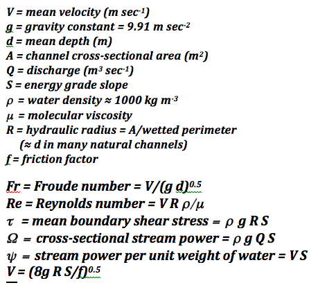
Fr is a dimensionless number that describes flow regimes in open channels and is unquestionably useful in many aspects of hydrology, geomorphology, and engineering. It is the ratio of inertial and gravitational forces:

Fr = V/(g d)^0.5

Fr < 1 indicates subcritical or tranquil, and Fr > 1 supercritical or rapid flow. But variations in Fr within the subcritical range (where it typically falls) can be significantly related to, e.g., geomorphic units and habitats within channels.

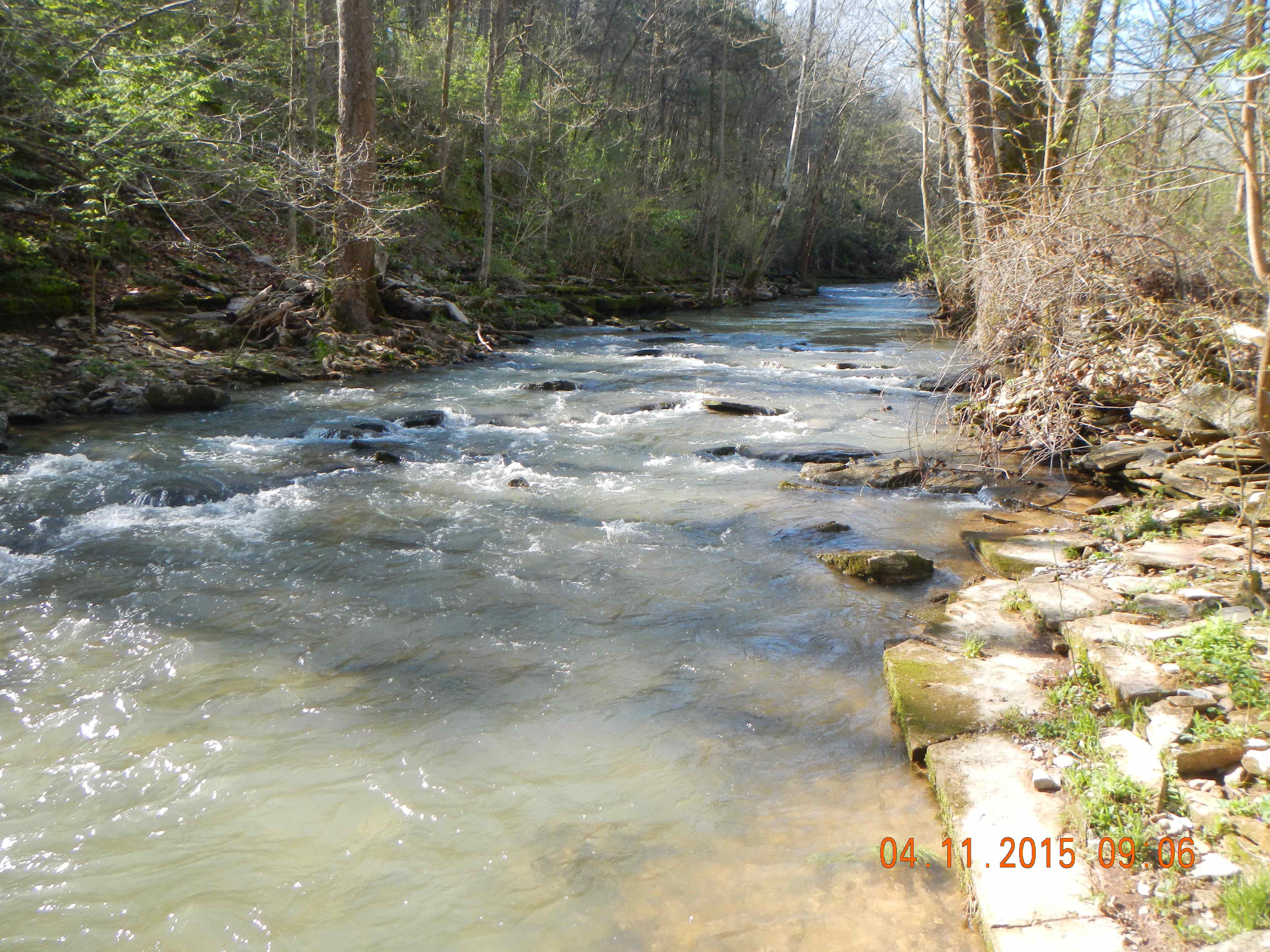
Shawnee Run, Kentucky

But what about other potential indicators? The Reynolds number (Re) is a measure of flow turbulence, shear stress (t) measures force exerted against channel boundary, and stream power indicates the rate of work or energy expenditure of flow. All of these, along with velocity or discharge, would seem to be as good or better indicators. So why is Fr so commonly employed?

If you take a look at the equations below, you can see that Fr varies directly and proportionately with velocity, and as the negative 0.5 power of depth. Reynolds number varies directly with V and d, and shear stress directly with d and slope. The stream power measures vary directly and proportionally with S and either V or Q. Thus, as flow conditions vary from wetter to drier periods and low to high flows, the Froude number is likely to be less variable than the other parameters. Thus, we can hypothesize that Fr is a preferred habitat indicator because it is more consistent.

My fluvial geomorphology class this semester tested this idea using field measurement data from U.S. Geological Survey gaging stations. These data include measurements of Q, V, channel width, and cross-sectional area. From these mean depth and the Froude number can be derived. They compared the coefficient of variation (mean divided by standard deviation) of Fr to that of discharge (related to cross-sectional stream power), V (related to Re and unit stream power as well as Fr) and d (related to Re and shear stress). A higher coefficient of variation (CV) for Froude number supports the notion that Fr is a preferred indicator because it is more consistent.

The students chose gaging stations representing a variety of fluvial settings, including bedrock-controlled, fluviokarst and alluvial channels; and high-gradient mountain and low-gradient coastal plain streams. Here’s what they found:

South Elkhorn Creek, Kentucky: The CV of Fr was greater than that for Q, d, and V for eight of the rating curves included in the data, with mixed results for three others.

Elkhorn Creek, Kentucky: : The CV of Fr was greater than that for Q, d, and V for all rating curves.

Dix River, Kentucky: The CV of Fr was greater than that for Q, d, and V for all rating curves.

Upper Cumberland River, Kentucky: The CV of Fr was greater than that for Q, but less than the CV of V and d.

Clear Fork, Kentucky: The CV of Fr was greater than that for Q, but less than the CV of V and d.

Cheat River, West Virginia: The CV of Fr was greater than that for Q, d, and V for all rating curves.

Lower Waccamaw River, South Carolina: The CV of Fr was greater than that for Q, and V and less than for d, for all rating curves. This site is tidally influenced, and d is almost constant as a consequence (less than 1 m variation for the entire data set).

Savannah River, Georgia/South Carolina (two stations near Augusta, GA): The CV of Fr was greater than that for Q, d, and V for six rating curves, and lower than Q, d, V for one rating curve.

Lower Colorado River, Texas (Bastrop): CV of Fr was greater than that for Q, d, but less than that of V for all rating curves.

Lower Colorado River, Texas (Bay City): The CV of Fr was greater than that for Q, d, and V for all rating curves.

Overall, results support the hypothesis that Froude number is less variable at a given location than other hydraulic indicators. Clifford et al. (2006) noted that different combinations of V and d could produce the same Froude number, and this was evident at many of the sites above. Many sites show bimodal relationships (i.e., two distinct trends) in relationships between Fr and V, Q, or d.

The data were also mostly low Fr. No value higher than Fr = 0.7 was recorded at any time at any station, and most values were less than 0.4 (many much less). Thus, sampling at smaller, steeper sites during high flows would be advisable for any future studies along these lines.

The students in the class who did the analyses are: Kornelia Wielisczko, Wisam Muttashar, Marielle Manning, Wei Ji, Jeremy Eddy, Sidney Dobson, and Darion Carden.

---------

Clifford, N.J., Harmar, O.P., Harvey, G., Petts, G.E., 2006. Physical habitat, eco-hydraulics and river design: a review and re-evaluation of some popular concepts and methods. Aquatic Conservation: Marine & Freshwater Ecosystems 16: 389-408. 

This is a continuation of a previous post, and this one will be even less intelligible unless you read that one first.

So, even though we rarely use the term, geoscientists have our metanarratives. Metanarrative is something of a perjorative for postmodern (pomo) critical social theorists, but just because because a metanarrative doesn’t really explain everything, even within its domain, doesn’t make it wrong, useless, or even hubris-y. As long we don’t make claims or insinuations, or have expectations, of a “theory of everything,” overarching theories or explanatory frameworks can be evaluated on their own merits or lack thereof—that is, whether a construct can be considered a metanarrative or not is independent of its utility and value.

The second thing pomos don’t like about metanarratives is that they tend to be global stories that overshadow, obscure, or misrepresent important aspects of local stories. Before I even heard of metanarratives and pretty much up to the present, I have been arguing for the importance of local, geographically and historically contingent factors in physical geography, geology, ecology, hydrology, and pedology (here are the earliest and most recent published examples). No matter how much data we obtain, we cannot explain everything based on universally applicable models, theories (or metanarratives) without marrying those to the contingent details of place and space. However, those same arguments assert that we cannot usefully base all our research in idiographic case studies—we need the overarching general principles (metanarratives?), too.

Some have interpreted my embrace of the local, and my critique of some geoscience metanarratives (particularly those based on balance-of-nature and normative equilibrium) as a postmodern attitude on my part. I’m not too concerned with how I get labeled, but please rest assured that I am not intellectually or academically aligned with the critical postmodern social theorists, though I count many as friends and colleagues. Metanarratives may be unhelpful, or repressive, but when this is the case it is not because they are metanarratives!

Now to another issue: I have suggested that some geoscience metanarratives based on equilibrium or optimality concepts are better explained as simpler emergent properties of Earth surface systems (see dis and dat). Is emergence, or selection, or historical/geographical contingency just another metanarrative? Are they meta² because they suggest that phenomena interpreted under a metanarrative of, e.g., dynamic equilibrium is a special case?

I don’t know and maybe I don’t care. What I do know is that the metanarratives I prefer and promote (if metanarratives they be) are attractive based on a classic, traditional scientific criterion: they are (or at least appear to me) to be the simplest possible way to explain observations. 

At my job I am housed in a building occupied mostly by social science and humanities scholars, many of whom are postmodern, post-structuralist, “critical” social theory oriented. The “critical” is in quotes not to cast aspersions, but because these folks use the term somewhat differently than do scientists, for whom all well-conceived legitimate work is critical in the sense of skepticism, testability, and the potential for falsification.  Anyway, my office location ensures that I am exposed to a good deal of the concepts and jargon of that community.

One of those is metanarrative. According to the Sociology Index web site:

Metanarrative is a story, narrative or theory which claims to be above the ordinary or local accounts of social life. Postmodernists claim that the majority of the writings of Karl Marx, David Emile Durkheim and Max Weber are offered as metanarratives, presented as capturing universal properties of social life and thus superior to local or more grounded stories. Postmodernist social theorists argue for a return to the local, the rejection of grand theory and a privileged position for science and its narratives, and an acknowledgment of the inherently political nature of all narratives. (http://sociologyindex.com/metanarrative.htm)

Some within the social science/humanities community argue that the pomos themselves construct metanarratives (for example of science) in their arguments. Notwithstanding that, I got to wondering about the metanarratives of the Earth and environmental sciences.

Hey, hope I'm not offending anyone . . . :)

Actual use and definitions of the term metanarrative seem to be confined to the “critical” social sciences and humanities, but if we think of them as narratives about narratives, or overarching stories that encompass or circumscribe individual stories, the idea is certainly applicable to the geosciences. Plate tectonics, evolution by means of natural selection, steady-state equilibrium, and balance-of-nature are all examples of metanarratives used (for good or ill) in Earth and environmental sciences.

Pomos, as best I can tell, don’t like metanarratives because:

1. They obscure or distort important local, case-specific aspects (not necessarily just details).

2. They are not universally applicable and do not explain everything within their domains.

The first critique is entirely applicable to geoscience metanarratives, though this doesn’t necessarily make the metanarratives wrong or useless. The second item, while undoubtedly true, is not a good reason for rejecting metanarratives. For example, the conservation laws for energy and mass are universally applicable (arguably THE only laws that absolutely must apply everywhere and always), but even in problems of say, sediment transport or fluid dynamics they don’t always explain everything. That fact does not deny the truth or diminish the utility of the conservation laws.

You have to be at least two different kinds of nerd to get this joke ( photo: https://unstruck.wordpress.com)

This discussion is continued in part II, next blog entry. 

A lot of us in the geoscience business are concerned these days with interpreting ongoing and past, and predicting future, responses of landforms, soils, and ecosystems to climate change. As one of my interests is rivers, I have noted over the years that in a lot of the literature on paleohydrology the major changes, such as major influxes of sediment, seem to occur at climate transitions, rather than after climate changes or shifts have had a chance to settle in and exert their impacts for awhile.

A related issue is the relationship between precipitation, temperature, runoff, erosion, and vegetation. As climate changes both temperature and precipitation regimes change. And as every physical geography student knows, moisture availability is not just about precipitation, but the balance between precipitation and evapotranspiration (ET). So, if both temperature and precipitation are increasing (as is the case on average on much of the planet now), whether available moisture increases or decreases depends on the relative increases of precipitation and ET.  

Soil erosion on cropland.

Increases in available moisture, also called effective precipitation, would tend to promote both runoff and soil erosion on the one hand, and vegetation cover on the other. Since vegetation reduces erosion, we have another case of the result hinging on the net effects of “competing” processes. So, how does this all play out?

The two best ways to find out, in my view, are case studies of actual responses, and complex system models that directly address the networks of interrelationships. The former, as I mentioned, typically show major changes in rivers, and influxes of sediment, at climate transitions. For the latter, previous work (including some of my own, but mostly by others) suggests dynamical instability—that is, the network of interrelationships is such that changes to any part of the system (e.g., accelerated erosion, or change in vegetation cover) tend to persist and grow (within limits) over time, rather than a return to the pre-disturbance condition.

I decided to take another look, using a model slightly more complex than the vegetation-erosion interaction models (these predict that the system tends to “tip” to either a maximum vegetation/minimum erosion or a maximum erosion/minimum vegetation state, with intermediate states unstable). The model below, though, is less complicated than more elaborate models (again, including some of my own) that also include soil hydrologic properties, nutrients, and other factors. Those also typically indicate dynamical instabilities under many circumstances.

Interrelationships among soil erosion, runoff, and vegetation under conditions of changing effective preciptation. Green arrows indicate positive links, indicating that an increase or decrease in one component produces a change in the other in the same direction. Red arrows are negative links, characterizing relationships where a change in one component produces a change in the other in the opposite direction.

Many of the links are fairly self-evident—other things being equal, effective precipitation is positively related to both runoff and vegetation cover, vegetation reduces erosion, and vice-versa (due to loss of topsoil, nutrients, etc.). Erosion also tends to increase runoff, due to reduced soil moisture storage capacity and exposure of low-permeability subsoils.

I actually prefer these qualitative (links are simply positive or negative) models, as they are more general than quantitative ones. For example, the quantitative effect of runoff on soil erosion varies with topography, soil factors, etc., and is more or less unique for a given situation. The qualitative relationship, however—runoff goes down, soil erosion goes down, and vice-versa—is more or less universal.

Anyway, the dynamical stability of models such as this can be analyzed mathematically (remember, qualitative ≠ non-mathematical) using the Routh-Hurwitz criteria. I’ll spare you the details (if you are interested, shoot me an e-mail), but the results are that the network of relationships are dynamically unstable.

From the perspective of climate change, that means that if a change in effective precipitation results in a change in vegetation cover or surface runoff, the effects of that change are likely to persist and grow (perhaps disproportionately large compared to the original change). This explains why paleohydrological studies typically show major changes or regime shifts during climate transition periods. Those changes in an unstable system generate disproportionately large responses in sediment dynamics.   

There’s an obvious warning here with respect to ongoing and future climate change—relatively minor climate-driven disturbances could result in disproportionately severe erosion and land degradation. But there’s also opportunity—in some situations relatively minor climate-driven disturbances in areas already experiencing erosion or degradation could be tipped into a minimum erosion, non-degrading state. And even in the former case, opportunities exist in such unstable systems to initiate relatively large desirable changes with relatively small “disturbances” such as, e.g., vegetation plantings or erosion control measures.

Eroded and restored gullies in Ethiopia (https://pcwoolner.files.wordpress.com/2013/02/mscfso.jpg). 

This is a continuation of my earlier post on applying state-and-transition models (STM) to stratigraphic information, to account for the missing bits.

Barrell’s (1917) explanation of how oscillatory variations in base level control the timing of deposition. Sedimentation can only occur when base level is actively rising. These short intervals are indicated by the black bars in the top diagram. The resulting stratigraphic column, shown at the left, is full of disconformities, but appears to be the result of continuous sedimentation. Noted sedimentologist Andrew Miall has used this example in several articles to illustrate the problems of gaps in sedimentary & stratigraphic records.

A stratigraphic record of paleoenvironments, for instance, indicates a number of different states. For example, a transgressive coastal sequence might have facies indicating nearshore, beach, dune, back-barrier, estuary, and freshwater swamp environments. These would represent the states in the STM, which are considered connected if one state can transition directly to another, with no intermediate states. Assuming for the moment a high degree of confidence in the STM, suppose one was faced with a sequence of beach sand overlying freshwater swamp peat. The STM could tell you whether such a transition was possible or likely, or whether intermediate states such as backbarrier marsh or open-water estuary must have existed, but are not preserved in the record.

How does one build stratigraphic STMs? STMs applied to problems in contemporary environmental change are based on a combination of monitoring, observation, historical reconstruction, modeling, and theory. For stratigraphic STMs, once reasonable states are identified, we might use a hierarchy of evidence to establish whether transitions can occur from state A to state B.

1. Theoretical plausibility. Given our knowledge of applicable laws and principles, is it (a) plausible, and (b) likely, that the AàB transition could occur. In many cases this can be explored via simulation models.

2. Stratigraphic evidence. If AàB can happen, then there should exist stratigraphic evidence (ideally in multiple samples) that this has occurred.

3. Observational evidence (modern analogs). The strongest form of support is field measurements or observations that the transition has occurred.

A good STM not only records what transitions are possible, but what causes or drives them. In the example below, for instance, specific geomorphic and pedologic processes are identified that drive the soil changes depicted.

Soil geomorphic state transition model for an agricultural landscape in the N.C. coastal plain (from Phillips, 2014).

OK, now suppose you have a sedimentary sequence that shows low marsh overlying alluvial crevasse splays, and your interpretation is guided by the STM shown below (which I have high confidence in, because I developed it!). This shows that in this environment, you cannot transition directly from crevasse splay to low marsh, and indicates that at least one intermediate stage is missing. The STM also indicates that, because of the various, interactive drivers of state changes in this system, the sequence one would expect if, say, only sea-level rise or increased sediment inputs were driving the system may not exist. But the absence of the sequence doesn’t necessarily mean the driver is absent!

STM for geomorphic environments in the San Antonio River Delta, Texas (from Phillips, 2014).

The STM framework is not a revolutionary technique for solving stratigraphic puzzles. Rather, it is a way of thinking about and analyzing environmental change that may be helpful to stratigraphers. In addition, this conceptual model is amenable to the analytical tools of graph and network theory, which could provide paleoenvironmental analysis with a new set of quantitative tools (see this previous post).

--------------------------------------------

Barrell, J. 1917. Rhythms and the measurement of geologic time. Geological Society of America Bulletin, 28: 745-904.

The reconstruction of past environmental change is more important than ever. First, we look for precedents, principles, and lessons from the past as we try to understand and predict ongoing and future environmental change based on the fundamental wisdom that “if it did happen, it can happen.” Second, all kinds of new ideas on the coevolution of life, landforms, climate, and Earth itself need testing, verification—and maybe most importantly—hypothesis generation from the historical record.

The most important historical records for all but the past couple of centuries are stratigraphic. Environmental change is recorded in the sedimentary rock record, in geologically modern sedimentary deposits, and in soil layers. However, geoscientists have long realized that the stratigraphic record is incomplete—“more gap than record,” Derek Ager famously pointed out, with the preserved events equally famously termed “frozen accidents.” The current state of affairs is well summarized in and recently published volume titled Strata and Time: Probing the Gaps in Our Understanding (Smith et al., 2015).

Stacked paleosols overlain by limestone in the Flint Hills of Kansas (image source: http://www.scifaithkansas.net/guide/FlintHillsGuide4.html)

As the book notes, a number of statistical and analytical methods have been developed to confront the fact that stratigraphic evidence often indicates apparently adjacent (in the stratigraphic column) events that are actually separated by long periods where little or nothing happened, and any number of events or episodes that were not preserved or were erased by erosion.

I’ve been working the past few years with state-and-transition models (see this and that). These are essentially box-and-arrow models that show the state, stage, or condition of an environmental system (e.g., landforms or soil types; vegetation communities; modes of landscape evolution) and the possible transitions among them. Could this approach be applied to the stratigraphic record? I think it is worth a try, and I will flesh this out a bit in my next post. 

State-and-transition model for geomorphic environments in the San Antonio River Delta, Texas (from Phillips, 2014). 

Wolfgang Scwhanghart, Tobias Heckmann and I have collaborated recently to review applications of graph theory in geomorphology and the geosciences in general. One of our papers, Graph Theory in the Geosciences, was just published in Earth-Science Reviews. The abstract is below. Our other joint paper, dealing specifically with graph theory applications in geomorphology, is still in press (in the journal Geomorphology) even though it was completed and accepted before the ESR paper. Go figure. 

What is the relationship between the diversity of resources (e.g., space, sunlight, water, nutrients) and biodiversity? In most cases it is direct and positive—that is, the greater the diversity of resources the greater the biodiversity.  The relationship is also often mutually reinforcing—that is, byproducts, detritus, and the organisms themselves increase the diversity of the resource base. Of course, ultimately both resource and biodiversity are limited by both abiotic and biotic controls. The relationships look something like this:

I analyzed a model of this same type, involving geomorphic systems, here. The upshot is that when the mutually reinforcing interactions between resource and  biodiversity are stronger than the abiotic and biotic limits on diversity, the system is dynamically unstable. This indicates that changes are likely to persist and grow over time, rather than to be offset. From the diversity perspective, this can be good—a small, local rise or surge in resource or biotic diversity would disproportionately increase overall diversity (e.g., gap dynamics in forests). However, it can also be bad—a decline in either can trigger an overall spiral of decline (e.g., effects of surface mining).

The resource diversity-biodiversity feedbacks will indeed be dominant, for good or ill, when an environmental system is well shy of its biotic or abiotic limits. As those limits are approached however, those negative arrows in the figure become dominant and the system is dynamically stable. That means that the effects of not-too-large changes or disturbances are offset or damped, returning the system toward its original state. Thus neither resource diversity nor biodiversity can increase indefinitely. Assuming the limits also work on the lower end—that is, there are always a minimum variety of resources available for some biota, even if only microbes, and a minimum variety of biota to exploit them—this also prevents extinction of biodiversity or complete vanishing of resources.

The implications of these dynamics for geomorphic systems are discussed in the article I referred to earlier. With respect to biodiversity, the restrictions on development in one direction or another are likely more variable and arguably less well known than for geomorphology, where factors such as base level and sedimentary accommodation space provide clear limits. Biodiversity involves different biota, of course, with different needs, tolerances, and sensitivities to various resources. Other than some obvious outer limits such as finite space and solar input (and photosynthetic efficiency), what are the bounds to diversity at the community level?

Studies of ecosystem engineering and niche construction may be extremely helpful in this regard. Introduced (invasive) species that are ecosystem engineers may provide opportunistic experiments where interrelated changes in resource and biodiversity may be observed.