The characteristics of a place or system can be factors that are measurable or observable, or those that are not observed or observable. Of the observable phenomena, there are (at least) two different classes. First, there are those whose detection and interpretation does not vary among observers (allowing, of course, for the fact that among us there are humans exceptional in various ways). But the vast majority of humans beyond infancy will recognize, say, a rock, and will not be inclined to argue about whether or not the boulder in question is a rock or not. Suitably trained observers (e.g., geologists) may further agree that the rock is, say, granite.

Some observable phenomena are such that their detection and/or interpretation may be highly sensitive to the characteristics of the observer. A relatively planar topographic surface, for example, may escape the notice of those not trained in geography or geology or experienced in observing landscapes. Geoscientists observing the same surface may disagree about its erosional or depositional origin, or if it is agreed to be an erosion surface, whether it is fluvial, marine, or some other origin. Even if the identification and characterization of a phenomenon is agreed upon, its meaning may be observer-dependent. Ecologists may agree that a forest stand is a late-successional stage dominated by oak and hickory, for example, but their training, experience, and inclinations may lead to quite different conclusions about whether this represents a stable climax community that is an attractor state, a happenstance combination of plants responding to a given set of environmental controls, a historically contingent outcome of various environmental changes and perturbations, or other interpretations.

We can divide the unobserved or unobservable phenomena into at least three different categories. Some are known to exist, though they cannot be measured or detected. Membership in this category tends to vary with spatial and temporal scale in the sense that what is readily observed at one scale may be invisible at another. Observability may be also be dependent on, and thus vary with, technology and expertise. The genetic basis for natural selection, for instance, was not observable before the development of genetics, and is unmeasurable for those without appropriate expertise and infrastructure.  A second category is phenomena that are believed or hypothesized to exist. This category is also dynamic, as changes in measurement technology and perception can confirm or deny their existence. Finally, we must always assume that unknown and unimagined processes and controls may exist.

Flows of mass and energy occur along the steepest gradients of potentials or concentrations.  The principle of gradient selection is simply that features associated with these gradients persist and grow. Take, for instance, the redistribution of excess (i.e., more than the ground can absorb or retain) surface water. Hydraulic selection principles favor the most efficient paths, which we can generally interpret as the fastest pathways. Thus the steepest slopes and/or the routes with the lowest resistance to flow attract more water. The most efficient paths persist and prevail; less efficient options dry up.  For example:

Standard flow resistance equations are of the general form

V = f(R^aS^bf^-c)

where R is hydraulic radius (cross-sectional area divided by wetted perimeter; typically roughly equal to mean depth), S is slope (hydraulic gradient), and f is a roughness or frictional resistance factor. The exponents a, b, c < 1. For example, the D’Arcy Weisbach equation is

V = 8g R^0.5 S^0.5 f^-0.5

Thus flow pathways where water is concentrated (greater R), slope is steeper (greater S) and resistance is lower (smaller f) are favored. Therefore concentrated flows (greater R, lower f) are favored over diffuse flows and steeper paths over gentler gradients.

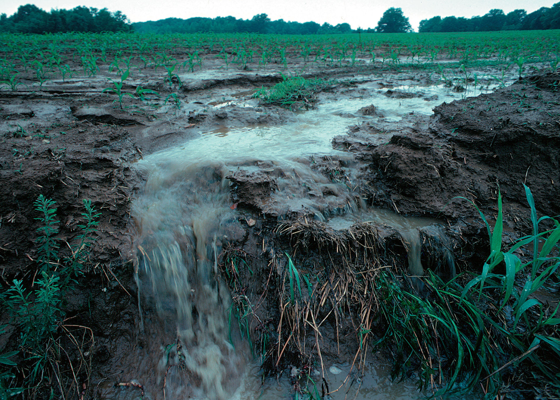
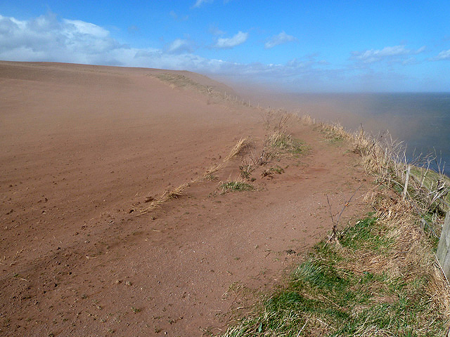
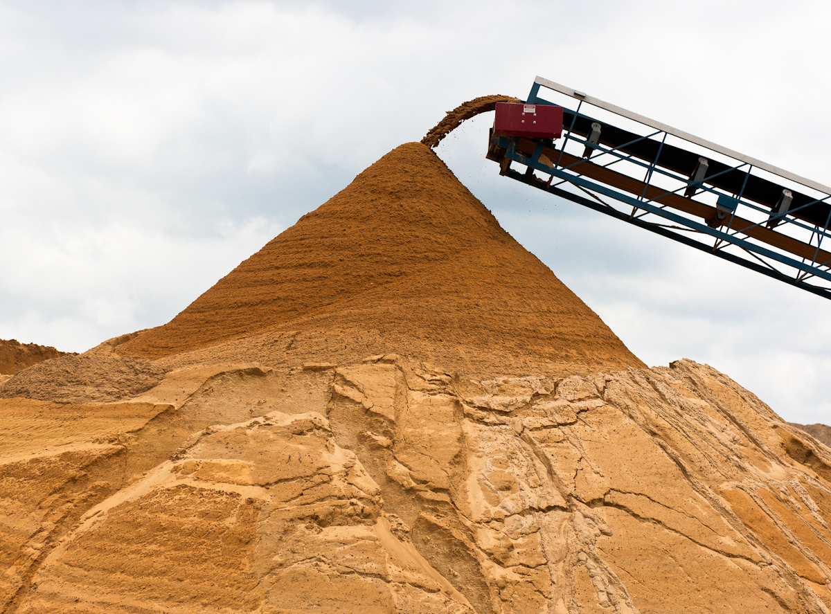
Gradient selection at work: even in flat topography concentrated flows tend to evolve and dominate (photo: L. Betts, USDA).

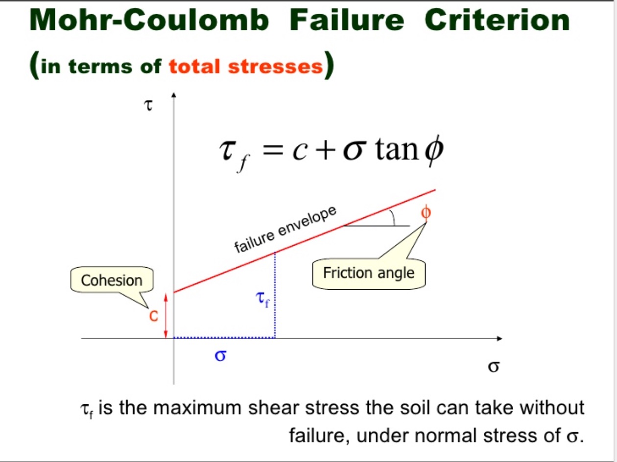
The force or shear stress exerted by a flow against its boundary is given by mean boundary shear stress (tau):

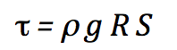
with rho the density of water, and g the gravity constant.  With R in m, tau has units of N m^-2.

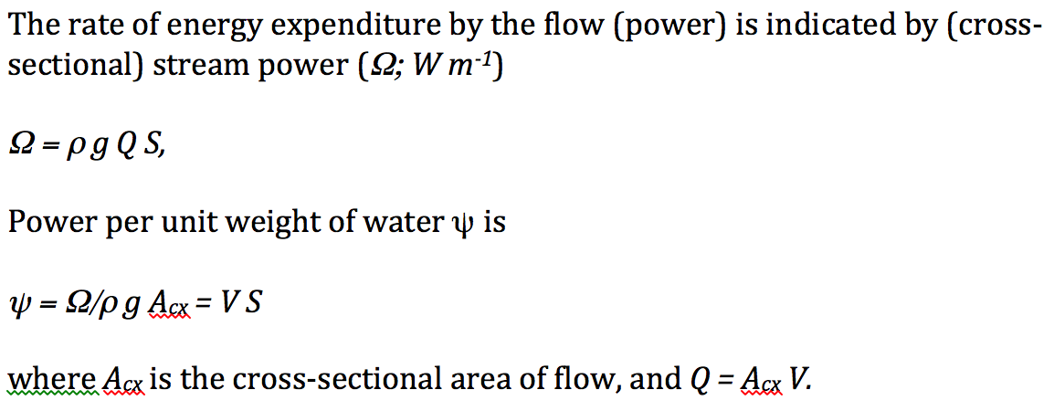
where A_cx is the cross-sectional area of flow, and Q = A_cx V.

Hydraulic selection favors pathways with faster V, and also deeper R, and steeper S. Thus hydraulic selection also tends to locally maximize shear stress and stream power. This is not a goal function or a basic principle of fluid flows—rather it is an emergent property; a byproduct. There is no principle that runoff and stream flow seek to maximize local shear stress or stream power; rather that is a corollary of hydraulic selection, which in turn expresses ideas we knew from our earliest experiences as children, on a rainy day or playing in a stream—water follows the steepest slope or the path of least resistance.

The emergent local concentration of force and power means that, at least occasionally, force will be sufficient to scour channels. This provides positive feedback reinforcement to hydraulic selection, and channels tend to persist. Steeper, larger, and hydraulically smoother channels are favored over smaller, shallower, rougher, and more gently sloping ones.

I may (or may not) have been the first to describe this as hydraulic selection (a specific form of gradient selection; Phillips, 2010), but I was hardly the first to recognize this as a selection phenomenon. Twidale (2004: 170) characterized channel formation as a process of natural selection, and Nanson and Huang (2008) outlined a principle of “survival of the most stable” with respect to channel configurations.

The "constructal law" of Bejan (2007) expresses basically the same idea as gradient selection: “For a flow system to persist in time (to survive) it must evolve in such a way that it provides easier and easier access to the currents that flow through it." Bejan (2007) provides examples of natural phenomena that illustrate this type of development, including wedge-shaped turbulent shear layers, jets and plumes, the frequency of vortex shedding, B́enard convection in fluids and fluid-saturated porous media, dendritic solidification, and coalescence of solid parcels suspended in a flow.

Michael Woldenberg derived these principles for channelized water flows in 1969 (Woldenberg, 1969). Lin (2010) critically reviewed literature on the prevalence of preferential flow paths of water at a wide range of scales, and the tendency for these to either be controlled by, or to evolve into, morphological features in soils and landscapes. By coupling traditional path-of-least-resistance reasoning to persistence of preferred flow paths, constructal-type behavior emerges, though Lin (2010) pointed out that constructal theory does not address the fact that flow patterns in natural hydrologic and pedologic systems are often strongly influenced by factors other than the flow itself.

Surface water flow is an archetypal example of gradient selection, but numerous other examples exist, including subsurface flows and associated processes. Water moves along paths of least resistance such as rock joints, macropores, faunaul burrows, zones of higher hydraulic conductivity, etc. Weathering, dissolution, erosion, and sediment transport within these features enhances these pathways at the expense of other nearby zones. This can occur even in homogeneous materials due to unstable growth of minor initial variations in moisture content. This results in unstable wetting fronts, fingered flow, and other preferential flow phenomena, which are manifested not only at the event scale, but often influence regolith and landform development (Dekker and Ritsema, 1994; Liu et al., 1994; Phillips et al., 1996; Ritsema et al., 1998; DiCarlo et al., 1999; Lin, 2010). The work of Heckmann and Schwangert (2013) indicates comparable phenomena at work on other hillslope processes, such as landslides and mass wasting.

The way water forms fingers in homogeneous sandy soils. Images are produced by passing light through sand and converting the different intensities to different colors (black = low moisture content; red = saturation) (http://soilandwater.bee.cornell.edu/Research/pfweb/educators/intro/fingerflow.htm)

Over time scales several orders of magnitude faster, air flows follow the “topography” described by isobars, which determine pressure gradients. Wind velocities are higher and air movement is greater where pressure gradients are greater, and vice-versa. Positive feedbacks also occur in these phenomena, as observed in the strengthening of high and low pressure systems, but these run their course in a matter of hours or days.

Resistance selection

Gradient selection as described above can be thought of as positive selective processes, dominated by less resistant paths of flow or change, and positive feedback, which reinforces changes associated with evolving flux pathways. Resistance selection, by contrast, is a negative form of selection dominated by resistant or repellent features, resulting in the persistence of more resistant forms or features. The principle of resistance selection simply states that more resistant features (relative to applied forces, or more generally, drivers of change) are selected for preservation, while less resistant components are preferentially lost or modified.

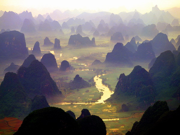
Resistance selection is closely related to, and in some cases simply an inverse way of describing or conceptualizing, gradient selection. Both reflect the effects of variations in the ratio of force (or other drivers of change) to resistance. In some landscapes, however, the resistant residuals--for example karst towers, or the ridgetops in dissected plateaus--rather than the preferred flow paths are the most obvious landscape characteristic. For our purposes, however, resistance selection is considered to be a subset of gradient selection.

Natural selection

The most famous notion of selection in nature is, of course, the principle of biological evolution by means of natural selection, originally articulated by Charles Darwin and Alfred Russel Wallace. Because of this, some object to the use of selection terminology in other scientific contexts. The use of the term “selection” here in gradient and resistance selection is not meant to imply any analogy between mass flux and landscape change phenomena with organisms. In some cases biota are critical components of the latter, and in some instances organic metaphors may be helpful, but please recognize that differences between, e.g., stream channels or soils and organisms in no way invalidates the application of selection concepts to the former. That is, I ask you to concede that use of the word “selection” does not have to be restricted to biological and organic phenomena. In fact, I searched for a different word, but my thesaurus yielded only “choice,” which carries teleological or anthropomorphic baggage we don’t want.  

In common with biological natural selection, gradient and resistance selection are emergent properties, arising from tendencies for certain configurations to persist, and for others to decline. I claim no other similarities.

Canalization and contingency

Once gradient or resistance selection has caused a particular configuration or pathway to be favored, positive feedbacks often reinforce it, as described earlier. This in turn often leads to a type of historical contingency called canalization. Once a channel is scoured or a canal constructed, this profoundly effects (and constrains) future water flows. The idea of canalization is that historical contingencies—for example evolutionary pathways, or development of structural relationships—direct future developments. Canalization originally appeared in evolutionary biology with respect to the notion of genetic canalization enhancing stability (Waddington, 1942), but the concept was subsequently broadened.

Levchenko and Starobogatov (1997) discussed canalization with respect to biological evolution. The previous development of biological systems prohibits some trajectories, and preferentially favors others. More specifically, they argue that the biosphere canalizes evolution independently of abiotic factors. Levchenko (1999) provided more detailed examples based on energy flows in evolutionary dynamics. Could this be a more direct link between gradient selection and biological selection?

--------------------------

Bejan, A., 2007. Constructal theory of pattern formation. Hydrology and Earth System Sciences 11, 753–768.

Dekker, L.W., Ritsema, C.J., 1994. Fingered flow: the creator of sand columns in dune and beach sands. Earth Surface Processes and Landforms 19, 153–164.


DiCarlo, D.A., Bauters, T.W.J., Darnault, C.J.G., Steenhuis, T.S., Parlange, J.-Y., 1999. Lateral expansion of preferential flow paths in sands. Water Resources Research 35, 427–434.


Heckmann, T., Schwanghart, W., 2013. Geomorphic coupling and sediment connectivity in an alpine catchment - exploring sediment cascades using graph theory. Geomorphology, 182, 89-103.

Levchenko, V.F., 1999. Evolution of life as improvement of management by energy flows. International Journal of Computing Anticipatory Systems 5, 199-220.

Levchenko, V.F., Starobogatov, Y.I., 1997. Ecological crises as ordinary evolutionary events canalised by the biosphere. International Journal of Computing Anticipatory Systems 1, 105-117.

Lin, H., 2010. Linking principles of soil formation and flow regimes. Journal of Hydrology 393, 3–19.


Liu, Y., Steenhuis, T.S., Parlange, Y.-S., 1994. Formation and persistence of fingered flow fields in coarse grained soils under different moisture contents. Journal of Hydrology 159, 187–195.


Nanson, G.C., Huang, H.Q., 2008. Least action principle, equilibrium states, iterative adjustment and the stability of alluvial channels. Earth Surface Processes and Landforms 33, 923–942.


Phillips, J.D. 2010. The job of the river. Earth Surface Processes and Landforms 35: 305-313.

Phillips, J.D., Perry, D., Carey, K., Garbee, A.R., Stein, D., Morde, M.B., Sheehy, J. 1996. Deterministic uncertainty and complex pedogenesis in some Pleistocene dune soils. Geoderma 73: 147-164.

Ritsema, C.J., Dekker, L.W., Nieber, J.L., Steenhuis, T.S., 1998. Modeling and field evidence of finger formation and finger recurrence in a water repellent sandy soil. Water Resources Research 34, 555–567.

Twidale, C.R., 2004. River patterns and their meaning. Earth-Science Reviews 67, 159–218.

Waddington, C.H., 1942. Canalization of development and the inheritance of acquired characteristics. Nature 150, 563-565.

Woldenberg, M.J., 1969. Spatial order in fluvial systems: Horton's laws derived from mixed hexagonal hierarchies of drainage basin areas. Geological Society of America Bulletin 80, 97–112.

Threshold modulation

Upper and lower limits

In terms of mass balances or budgets, geomorphic systems have three fundamental states, whereby losses or removals are either greater than, less than, or roughly equal to inputs or gains (i.e., steady-state). Thus a regolith cover, for instance, is either thinning, thickening, or maintaining steady-state relative to the rates of mass losses and inputs, and weathering and regolith formation.

The principle of threshold-mediated modulation holds that thresholds limit development on both ends (negative or positive mass balance), and that exceeding the thresholds may initiate development in the opposite direction. For instance, vertical accretion on alluvial floodplains is limited by an elevation at which regular flooding no longer occurs, thus limiting further accretion. In addition, confinement of flows within the channel may increase stream power and shear stress, thus ultimately resulting in stripping of the alluvium.

A specific example discussed by Phillips and Lutz (2008) is stream channel slope. While reverse slopes and overhangs may occur at the local, cross-section scale, at a reach scale geotechnical properties of the bed material in the landscape context determine a maximum slope gradient that can be maintained. At lower slopes, some minimum gradient is needed to maintain downstream water flux. Within a reach, gradients anywhere between the limits are possible, and exceeding the gradient thresholds results in adjustments (slope failures or ponding) that modify channel slopes away from the limiting gradient.

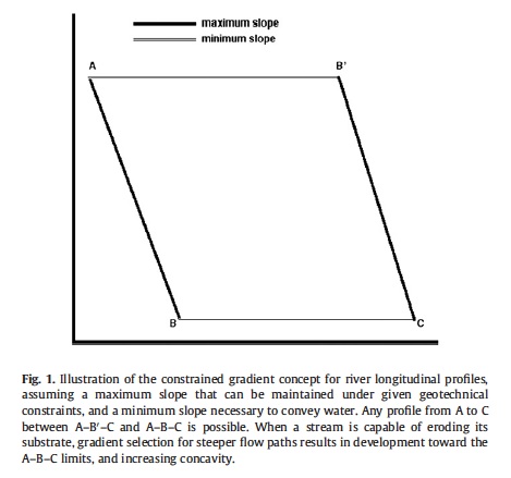
From Phillips & Lutz, 2008

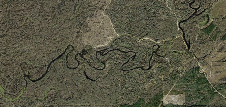
Thresholds are in some cases defined (or are non-trivial) at only one extreme. The angle of repose as a threshold of steepness for hillslopes is one example, with thresholds of minimum slopes generally zero (flat). However, where clearly defined thresholds exist for both the positive and negative cases, oscillation between these may appear to be constrained around a central tendency rather than by the extremes.

For example, imagine a frictionless pendulum swinging back and forth at a constant rate along a constant path. The path and position are constrained by the extremes of the arc, not by the central, vertical position, and no position or direction between the endpoints is more common, characteristic, or normative than any other. If the position of the pendulum and its direction of movement is measured at frequent but random intervals, the mean position will be the vertical position at the bottom of the arc. If this were interpreted as a normative equilibrium, then it would appear that movement away from this point is limited, and half the time the system would be moving toward this point. This is an example of apparent, pseudo-equilibrium, where observations are consistent with the notion of tendencies to return to a single normative state even though the behavior is actually characterized by oscillation between extreme states. The pendulum metaphor is not meant to imply a direct analogy to equilibrium concepts in geomorphology. Rather, the intent is to illustrate how a halfway position in a cyclic or oscillating system could be misinterpreted as an attractor or equiilibrium point. 

In alluvial rivers, for example, aggradation is ultimately limited by reduced floodplain accretion (as described above) and eventual flood stripping or bank failures if floodplain accretion exceeds channel accretion (Nanson, 1986) or by avulsions if channel accretion is greater than or equal to floodplain upbuilding. Incision-dominated degradation is ultimately limited by local base level and minimum slope requirements, and may be limited short of those extremes by exposure of bedrock or other resistant materials. Laterally-dominated erosion is eventually checked by valley side slopes and valley confinement, or by sinuosities so great that cutoffs become inevitable (Hooke, 2003; 2004). Neither aggradation nor degradation can continue indefinitely, even if external drivers such as tectonics, climate, or sea-level are constant.

Tortuous meanders & cutoffs, Old River, Beauregard Parish, LA (Google Earth image)

In most alluvial rivers, net aggradation or degradation is the norm, and steady-state is rare and transient. The transitions from one state to the other, and the approach toward and achievement of steady state during these transitions (analogous to the pendulum swinging from one end of the arc back to the middle) do not represent any inherent tendency toward the steady-state condition, but merely a byproduct or emergent property of the oscillations between aggradation and degradation.

With respect to regolith thickness, while the thresholds limiting the upper limits are less clear, and oscillatory behavior appears less common, thicknesses may also vary from steadily increasing thickness to complete regolith stripping, with evidence for steady-state relationships (addition of new material by weathering or input via deposition roughly equals removals) relatively uncommon (see Phillips, 2010b and references therein).

Critical Limits

In some geomorphic systems thresholds limit the amount or rate of change, or the accumulation of potential energy, but at the other end of the continuum the feature or phenomenon may simply disappear or become irrelevant. For instance, rates of karst dissolution, even where water and CO₂ are not limiting, are ultimately limited by Ca concentrations and aggressiveness of the water and other limits on weathering kinetics (Dreybrodt and Gabrovsek, 2002). There are no feedbacks preventing reduction of dissolution rates to zero, however.

Tower karst, Guangxi, China (photo: http://science-junkie.tumblr.com/post/42590142332/)

In some of these systems, such as karst, no relevant steady-state equilibrium (SSE) condition exists. While locally dissolution and precipitation may be balanced, in terms of landform and landscape evolution there exists only a continuum from the upper limits on the rate of karst processes and the extent of development of karst landforms, to rates of zero. In others the steady-state condition (e.g., shear strength = shear stress on a hillslope) represents one of the limiting extremes.

Thus steady-state may represent an intermediate point in some geomorphic systems (e.g. aggrading/degrading rivers; thickening/thinning regoliths), an upper limit in others (e.g., slope angles), and be irrelevant in still others (e.g., karst landscape evolution).  SSE therefore seems an inappropriate concept to represent normative behaviors or modal tendencies of earth surface systems in general.

Note: I previously dealt with threshold modulation in this article.

------------------------------------------

Dreybrodt, W., Gabrovsek, F., 2002. Basic processes and mechanisms governing evolution of karst. In: Gabrovsek, F. (Ed.), Evolution of Karst: From Prekarst to Cessation. Zalozba ZRC, Ljubljana, Slovenia, pp. 115–154.

Hooke, J.M., 2003. River meander behavior and instability: a framework for analysis. Transactions of the Institute of British Geographers 28, 238–254.

Hooke, J.M., 2004. Cutoffs galore! Occurrence and causes of multiple cutoffs on a meandering river. Geomorphology 61, 225–238

Nanson G., 1986, Episodes of vertical accretion and catastrophic stripping: A model of disequilibrium floodplain development, Geological Society of America Bulletin, 97: 1467-1475

Phillips, J.D., Lutz, J.D.  2008.  Profile convexities in bedrock and alluvial streams.  Geomorphology 102: 554-566.

Phillips, J.D.  2010.  The convenient fiction of steady-state soil thickness. Geoderma 156: 389-398.

If Mother Nature has plans, those plans are flexible. She keeps her options open, allows for more than one route to a given location, and we cannot assume that the same circumstances will always produce the same outcome. To digress for a moment: accepting this need not challenge religious or philosophical beliefs about a creator. Nothing in the bible, for instance, specifies exactly how the Judeo-Christian God goes about his/her business, or specifies any single pathways or mechanisms. As a protestant minister I knew well used to say: “Religion is concerned with the ‘why’ questions, and science addresses the ‘how.’”

Indeed. 35 years in the geoscience research business has shown me that that there is no single “right” or “natural” way for the world to be. Any human notions of singular, immanent norms or optima are tied to needs, goals, or perceptions, not scientific laws or relationships. And—again—there is nothing wrong with having such goals, desires, or expectations for nature, any more than there is anything wrong with a farm or a garden. The key is to realize that there is not much point in expecting Earth surface systems to evolve toward and maintain a single specific condition, any more than we would expect a garden to maintain itself without some guidance and intervention.

Why, then, in the face of overwhelming evidence to the contrary do people, scientists and laypersons alike, adhere to worldviews, conceptual frameworks and models based on singular, normative states of Earth systems?

My best guess is based on two propositions: (1) Humans want to impose (or imagine) order and predictability on nature; and (2) certain aspects of environmental systems imply a “balance of nature;” particularly to those (most) of us predisposed to believe in or desire it.

Jonesin’ for Order

Why do we want to find or impose order and predictability in nature? Most fundamentally, I think, it is because creation is vast, complicated, and complex. We have no hope of even getting our heads around it (or parts of it) intuitively, much less achieving any scientific understanding, without simplifying it in some way. Assuming or postulating a normative state is one way of doing this, and a “balanced” state is as good a choice as any and better than most, since it is quite often a logical reference condition, regardless of attitudes about normativity.

There also exists, of course, abundant evidence that hardwiring in our brains and cultural conditioning both compel us to seek orderly patterns. There are neurological, psychological, social, cultural, aesthetic, and pragmatic aspects to this compulsion that are way beyond my expertise. However, I am well convinced that this compulsion exists, in varying degrees and manifestations, in all of us.

Normative equilibria and balance of nature concepts are also often a matter of convenience or practical necessity. We can’t realistically manage rivers, farms, ecosystems or anything else without some sort of target or goal. Choosing these targets is a lot easier when we assume or imagine a single natural or balanced desired state. Conversely, justifying and explaining management goals is easier if you can claim to be doing exactly what nature intended. And sometimes, faced with multiple options and limited information, the assumed normative equilibrium state may be as good a choice as any.

Finally, as scientists, we emphasize what we do understand (or think we understand) and can predict. And balance-of-nature and equilibrium ideas and models do sometimes help us understand and predict. The underlying equilibrium assumptions may be unrealistic, or just plain wrong, but that doesn’t necessarily prevent them from being useful in some situations (I have written about this in the context of soil and fluvial geomorphology here, here, and here). I often use the analogy of the common economic modeling assumption that all participants always act rationally, in their own best fiscal interests, and with perfect knowledge. The fact that this assumption is untrue does not prevent the models from working well in certain situations.           

Keeping Up Appearances--of Equilibrium

So we want or need equilibrium and balance, or at least find it to be a convenient fiction. What is it about environmental systems that enable us to think we see it when it is not there, or to think that a balanced state is more normal or common than otherwise, rather than just one of several possible conditions?

First, consider relaxation time equilibrium. Relaxation time is how long a system takes to complete its response to a change or disturbance. In Earth systems relaxation time is always finite, and very often decelerates. That is, the response is often rapid at first, and then quickly or gradually slows to negligible rates. This can readily be interpreted, if one is predisposed to do so, as the system achieving a new steady-state or normative equilibrium. The more likely and logical interpretation, however, is simply that relaxation time has elapsed, and that the new state was not necessarily preordained.

Second, Earth systems do often have buffering capacities, feedback mechanisms and multiple degrees of freedom in responding to changes. These do not necessarily always operate so as to restore or maintain a (single) balanced state, but they do, along with the first-order constraints imposed by general laws, constrain what can happen.

Third, some systems oscillate (not always regularly, of course) between different sorts of imbalance—for instance, aggradation vs. degradation in river systems. Where this occurs, the system must sometimes be in or near the balanced steady-state, and on average will be approaching this state about half the rest of the time. Interpreting this as a system somehow seeking steady state is like saying humans are seeking a state of partial wakefulness (just waking or falling asleep), but you can see it if you believe it.

Fourth, balanced states are often both scale and time dependent. That is, one can always make the focus either vast or tiny enough to find a state of balance, or find some period of history where balance obtains. Even in the most variable systems, you can zoom into ever-shorter periods (or smaller areas) where balance temporarily prevails, and over ever-longer time spans (or broader areas), things often even out. Further, given the long time scales for many Earth systems and the generally episodic nature of change, it is often easy to find times where little or no change is occurring. Therefore, if you really want to find steady-state, you can—I guarantee it.

Finally, as alluded to earlier, model assumptions based on balance-of-nature ideas are often useful, even when the assumptions are untrue.

Taken together, these aspects of nature can easily give an impression of a balance of nature to those who are looking for it.

How I Stopped Worrying and Learned to Love Nonequilibrium

Let me make clear—I am not saying that steady-state and other equilibrium conditions do not exist, or even that they are rare. I am saying that there are often multiple equilibria for a given environmental system, and that equilibria or steady-states are not in general more common, important, or “normal” than disequilibria and nonequilibria. Further, I happily acknowledge, and sometimes make use of, the convenient fiction of steady-state as a reference condition or simplifying model assumption.

Admitting that there is not, or may not be, a balance of nature, does not imply a lack of any kind of order, regularity, or predictability. It does change the context of predictability, but this can be dealt with, as a vast literature on complexity, nonlinear dynamics, nonequilibrium dynamics, multiple stable states, path dependency, and state-and-transition models in geomorphology, ecology, pedology, and other sciences shows.

There are certain aesthetic virtues to symmetry and orderly patterns. Belief in balance and order may bring some inner peace and reassurance. But far more compelling, to me, is the aesthetic joy one can take in the infinite variety of nature, and the fact that each landscape or ecosystem is in some nontrivial respects absolutely unique.

Heraclitus said “you cannot step twice into the same river.” Nature as we view it now or reconstruct it in the past is a historically contingent snapshot. There is no single way that it is or was supposed to be, and more than one possibility for the future. Our world is, therefore, like many of us: not simple to understand, but easy to love.

In 1997, world leaders met in Kyoto, Japan to discuss how to confront, combat, and adapt to climate change. Eighteen increasingly warmer (on average) years later, a new set of climate talks start in Paris (France, not Kentucky) today (30 November), and continue for 12 days.

Some U.S. politicians have already courageously declared that the U.S. will do nothing, no matter how compelling the evidence, how severe the problems, or what the rest of the world thinks. As we get a new round of public commentary during and after the Paris talks, two recent studies—one journalistic and one academic—are worth considering.

The academic study is an article recently published in the refereed scientific journal Climatic Change, by Syrdan Medimorec and Gordon Peacock, titled “The language of denial: text analysis reveals differences in language use between climate change proponents and skeptics.”  The authors examined the text of the most recent Intergovernmental Panel on Climate Change report, by a large international group of climate science and climate impact experts, and a competing assessment produced by politically conservative climate change deniers and skeptics. Despite the title of the article, by the way, the IPCC is not composed entirely of climate change proponents—it simply happens that the overwhelming majority of scientists recognize climate change and the risks associated with it. In general, the denier camp (the so-called skeptics), while increasingly unable to deny the reality of climate change, generally charges the climate science community with overstating the risks. However, Medimorec and Peacock found that it is the IPCC, not their critics, who are demonstrably more scientifically conservative and politically circumspect. The abstract of their paper:

We used text analyzers to compare the language used in two recently published reports on the physical science of climate change: one authored by the Intergovernmental Panel on Climate Change (IPCC) and the other by the Nongovernmental International Panel on Climate Change (NIPCC; a group of prominent skeptics, typically with prior scientific training, organized by the Heartland Institute). Although both reports represent summaries of empirical research within the same scientific discipline, our language analyses revealed consistent and substantial differences between them. Most notably, the IPCC authors used more cautious (as opposed to certain) language than the NIPCC authors. This finding (among others) indicates that, contrary to that which is commonly claimed by skeptics, IPCC authors were actually more conservative in terms of language style than their NIPCC counterparts. The political controversy over climate change may cause proponents’ language to be conservative (for fear of being attacked) and opponents’ language to be aggressive (to more effectively attack). This has clear implications for the science communication of climate research.

As illustrated by graphics like this, supporters of action to reduce climate change can also be guilty of hyperbole. However, the scientific assessments are generally conservative and not exaggerated. 

In the journalistic study, the Associated Press asked eight climate and biological scientists to assess what 12 U.S. presidential candidates said in interviews, debates and tweets about climate, grading them on a 0 to 100 scale. To minimize bias, the candidates’ comments were stripped of names and assigned random numbers, so the scientists would not know who made each statement they were grading. The participating scientists were also selected by scientific societies, not the AP.

If we assume a 10-point grading scale (90-100 = A, 80-89 = B, etc.), there were two A’s (Hilary Clinton, Martin O’Malley), one B (Bernie Sanders), one D (Jeb Bush), and eight F’s. Of the latter, Chris Christie led the way with a 54, while Donald Trump, Ben Carson, and Ted Cruz brought up the rear with grades of 15, 13, and 6, respectively. One scientist wrote of one unidentified test subject, who turned out to be Cruz: “This individual understands less about science (and climate change) than the average kindergartner. That sort of ignorance would be dangerous in a doorman, let alone a president.” The AP’s story is here.

I do not know enough about the individual candidates to judge their overall intellect and education, and I acknowledge that some may truly be dimwitted and uninformed. However, I cannot imagine that they all are, and can thus only hypothesize that they make statements that they know are false or misleading to please certain political and donor constituencies.

So, as you evaluate public statements coming out of, or about, the climate talks, I suggest you consider the sources! Meanwhile, consider that in the 18 years since the Kyoto meetings:

•The Greenland and West Antarctic ice sheets have lost 5 trillion metric tons of ice (Andrew Shepherd, University of Leeds).

•Earth set a record for its hottest year since record-keeping began in 1997—a record that was subsequently broken in 1998, 2005, 2010, and 2014, and is sure to be broken again once 2015 is done (U.S. National Oceanic & Atmospheric Administration).

•Glaciers have lost, on average, 12 meters of ice thickness (World Glacier Monitoring Service, Switzerland).

•Global carbon dioxide emissions have increased more than 50% (U.S. Department of Energy).

•Arctic sea ice coverage is on average more than 2 million km² less at its summer low point (U.S. National Snow and Ice Data Center).

•The five deadliest heat waves in history have occurred (in order of number of deaths, Europe 2003, Russia 2010, India & Pakistan 2015, western Europe 2006, southern Asia, 1998) (Centre for Research on the Epidemiology of Disaster, Belgium). 

Texas A&M University Press has recently published Texas Riparian Areas. According to TAMU Press's blurb: 

Riparian areas—transitional zones between the aquatic environments of streams, rivers and lakes and the terrestrial environments on and alongside their banks—are special places. They provide almost 200,000 miles of connections through which the waters of Texas flow. Keeping the water flowing, in as natural a way as possible, is key to the careful and wise management of the state’s water resources.

Texas Riparian Areas evolved from a report commissioned by the Texas Water Development Board as Texas faced the reality of over-allocated water resources and long-term if not permanent drought conditions. Its purpose was to summarize the characteristics of riparian areas and to develop a common vocabulary for discussing, studying, and managing them.

I authored two chapters -- one on stream buffers, and one on riparian geomorphology. There are also chapters on riparian soils, vegetation, management, and landowner assistance. These are framed by integrated overviews on riparian ecosystems, and management issues in the Texas context. 

Texas is a big place, with environments ranging from deserts to subtropical swamps, and a lot in between. Thus, even though the book's emphasis is on Texas, I think a lot of the book will be relevant elsewhere, too. 

You can order, or learn more about it, here.

For the past five years or so, I have been working on adaptations of algebraic or spectral graph theory to study geomorphic, pedological, and ecological systems. My most recent development (unpublished, for reasons that will become clear in a moment) is some methods for measuring the complexity of historical sequences in Earth surface systems.

The idea is that a historical sequence represents a series of different states or stages—for example, vegetation communities along a successional trajectory; river channel morphological states; different soils in a paleosol sequence; depositional environments in a stratigraphic sequence, nodes of phylogenetic trees in biological evolution, etc.  These are treated as directed graphs. The states or stages are the graph nodes or vertices, and the historical transitions are the edges or links between the nodes.

These kinds of sequences are most often conceptualized as linear progressions (A-->B-->C--> . . . .) or as cycles ((A-->B-->C--> . . . -->A). If that accurately represents the system, great—those are the simplest graph structures! However, in some cases the evolutionary sequence is divergent—it splits or forks, as in a biological evolutionary tree, cladogram, or phylogenetic sequence. Divergent evolution has also been documented recently in geomorphic and pedologic systems. Or in some cases, previously existing states reoccur in ways other than a simple cycle. In yet others, more complex mesh-type networks of various transitions among system states may evolve (this is best illustrated by the more complex state-and-transition models).

Algebraic graph theory allows us to measure the structural complexity of the historical sequence (via the graph spectral radius), the (inferential) synchronicity and convergence properties (via algebraic connectivity) and the extent that a subgraph is representative of the overall pattern of historical change, which can be useful if you know or suspect that not all relevant transitions have been observed or inferred. I can also determine the extent to which graph complexity is due to the number of possible transitions vs. the specific way the transitions are wired.

To me this seems like some great stuff. But, on the other hand, I am not happy with simply measuring or quantifying something because I can. What information or insight can quantifying the complexity of historical sequences of Earth surface system development gain us? What geoscience or ecological problems could it solve, or at least address?

That’s what I’m not sure about.

(http://ux.stackexchange.com/)

Abraham Maslow is often credited with the saying that if all you have is a hammer, every problem looks like a nail. Some geoscientists are guilty of this, I suppose, as are other scientists. More often, however, we get or devise a new hammer, metaphorically speaking. We realize that not every scientific problem is a nail, so we grab the hammer and go looking for a nail. That’s what I feel like now. If you know of a nail I might take a whack at with this hammer, or otherwise have thoughts on how this particular hammer might be useful, I’d love to hear from you (at jdp@uky.edu).

Some of my previous algebraic graph-theory based work on historical networks is available here and here. 

The standard conceptual model for pedology, soil geomorphology, and soil geography is often called the “clorpt” model, for the way it was portrayed in Hans Jenny’s famous 1941 book The Factors of Soil Formation:

S = f(cl, o, r, p, t) . . . .

This equation states that soil types or soil properties (S) are a function of climate (cl), biotic effects (o for organisms), topography (r for relief), parent material (p), and t for time, conceived as the age of the surface the soils are formed on, or the time period the soil has been developing under a given broad set of environmental controls. This factorial approach, considering soils as a function of the combined, interacting influences of environmental factors such as geology, climate, and biota, was originated by V.V. Dokuchaev in Russia in the 1880s, popularized in English by C.F. Marbut in the 1920s and 1930s, and developed by Jenny into the familiar clorpt form.

Much has been written about the state factor model, including a 50^th anniversary retrospective of Jenny’s book that addresses not only the model’s history and impacts on soil science, but also its impacts on geomorphology, geoarchaeology, geography, paleoenvironmental reconstructions, and ecology. My own take (from the 1990s) on the factorial model as a nonlinear dynamical system is here and here.

Note that the clorpt equation, when correctly displayed, always has some trailing dots. This was Jenny’s way of showing that, in any landscape, one should consider climate, organisms, topography, parent material and time factors, but that there are other factors (the “dot factors”) that are critical in some locations and situations, but not everywhere.

I’ve always thought the state factor model was a good general representation of geographical explanation, where multiple causality is the rule. That is, the phenomenon of interest is determined by multiple environmental (or in other contexts, perhaps economic, political, etc.) controls that may themselves interact. The representation with the dot factors is also dead on, in my view, because it reflects the fact that any Earth surface system is influenced by a set of general or universal factors that apply everywhere and always, and by a set of local or contingent factors that are specific to place and time. The dot factors can be thought of as representing the latter.

In days of old (i.e., when I was a student), aeolian deposition was often cited as a dot factor—significant in some areas but not everywhere. Now I think aeolian inputs are more significant over much of the planet than we once imagined, but that’s another story. I wanted to yap a bit about dot factors not only because of the intrinsic geoscience significance, but because with ongoing climate and other environmental changes we are likely to see dot factors in many environments change—wax or wane in relative importance; perhaps emerge or fade away.

For example, in the coastal zone salinity and sea level change are crucial soil-forming factors (I’ll stick to this term for brevity’s sake, but keep in mind that these are also critical geomorphic and ecological factors, too). As sea level rises, the effects of these dot factors will increase in importance over a broader area inland (and decrease seaward, as, e.g., salt marshes are eroded and drowned).

Wind erosion & deposition in the United Kingdom (www.geograph.org.uk).

Sediment redistribution by erosion and deposition is an important soil-forming factor, and in most landscapes is accounted for by “r”, as these are generally topographically driven. However, in some arid and semi-arid environments (and coastal sand dunes) wind is the major erosion and sediment transport agent, and of course aeolian processes, while influenced by topography, are driven by pressure gradients, not gravity. Climate change may well produce situations where such processes become both more and less active.

A Canadian cryosol with subsurface ice body (Agriculture Canada photo).

Cryosols in periglacial and tundra environments are affected by subsurface ice bodies. As permafrost thaws during global warming, these ice lenses will disappear. There is also strong evidence that climate change is influencing fire regimes (for instance, increasing fire frequency in the western US). Some impacts of fire could perhaps be incorporated in the organic factor of the clorpt equation, but fire has impacts on soils independently of its effects on vegetation and organic matter.

Sycamore tree penetrating and displacing bedrock in central Kentucky. 

The biotic or organic factor in the soil factor equation was originally viewed as primarily reflecting general correlations between soil type and vegetation cover, though the importance of other organisms is more widely recognized now. A common subject of my own research in recent years—and that of many others—is the effects of individual trees on soils, which can be considerable. It could be argued (I will not do so here) that this could, or could not, be incorporated into the “o” factor. However, in some cases these effects (e.g., uprooting) are closely related to disturbance events such as tornadoes, other windstorms, and ice storms; and pest infestations or other tree-killing events. These are all likely to be influenced by climate change, and perhaps best considered as local dot factors.

Other pedologists could no doubt add other examples. The main point is this—as climate changes, it is not just the cl factor in the form of temperature, precipitation, etc. that will change—in many cases the dot factors will change, too.

Nearly 10 years ago, while pondering complex nonlinear dynamics in geomorphic systems, I was struck by how often we reduce problems to the interplay of opposing forces (e.g. uplift vs. denudation; soil formation vs. soil erosion, etc). I began to wonder how the concept of dialectics might be applicable in Earth sciences, or maybe I just wanted to increase my pseudo-intellectual street cred by using "dialectics" in an article. Anyway, I started work on a manuscript with the working title shown above, and then dropped it. I rediscovered it on the hard drive recently, and while I still can't convince myself it is journal article material, I do think there's some potentially interesting ideas there. 

What you see below is what I wrote in early 2006 (thus the absence of reference to work since then), unmodified except for putting in a few graphics to relieve the visual tedium.

1. Introduction

The title begs at least three questions: what do I mean by dialectics, how am I defining complexity, and how do I propose to link them?

1.1.  Geomorphic Complexity

Complexity, like equilibrium, means different things to different scientists. The American Heritage Dictionary (2000) defines complexity as the quality or condition of being complex, which is in turn defined in its adjectival form as consisting of interconnected or interwoven parts. The scientific study of complexity, often linked with terms such as complexity theory, is often linked to nonlinear dynamics, self-organization, and other theoretical and methodological constructs. However, complexity in the common definition may not necessarily derive from chaos, criticality, or other sources. Various definitions of system complexity have been proposed. In this paper the complexity of a geomorphic system is considered to be a function of:

(1)  The number of elements or components.

(2)  The number of links or relationships among the elements or components.

(3)  The (non)linearity of the relationships.

(4)  Historical contingency and memory.

(5)  Spatial scale.

(6)  Temporal scale.

(7)  External forcings and constraints.

Other things being equal (though of course they never are), the larger the number of components and links between them, the higher the degree of nonlinearity, the more past states and events influence current states, and the greater the potential range of spatial and temporal scales or resolutions over which system dynamics are manifested, the more complex the system is likely to be. The extent to which the system is influenced by external factors, and the nature of those external factors, also influences system complexity, but it is impossible to generalize beyond that, as externalities may increase or decrease complexity.

This notion of complexity does not require nonlinearity, or any particular form of nonlinear dynamics. A system might be complex simply due to a large number of components and many degrees of freedom, and/or to variation across a broad range of scales. Likewise, complex geomorphic systems need not be high dimensional, if for example they are highly nonlinear and chaotic (implying contingency).

1.2.        Dialectics

Five definitions of dialectic(s) are found in the American Heritage Dictionary (2000). One is “the contradiction between two conflicting forces viewed as the determining factor in their continuing interaction.”  Given that geomorphologists often treat problems in terms of conflicting forces (weathering vs. erosion, force vs. resistance, uplift vs. downwasting, etc.), this definition is relevant to Earth sciences.

The other definitions are more or less related to analyses and critiques practiced in the social sciences and humanities and generally associated with Marx, Engels, and Hegel. One might speculate that accumulating a full hardcopy collection of writings on this subject in one location would result in a mass sufficient to trigger isostatic adjustment. Here we focus on Engels (1883) Dialectics of Nature, where he attempts to develop Marxian dialectics as the “science of interconnections.” In ch. 2, Engels puts forward three laws, following Hegel but with specific applications to the natural sciences:

i.               Transformation of quantity into quality;

ii.              Interpenetration of opposites;

iii.             Negation of the negation.

The first law states that gradual quantitative changes ultimately lead to turning points or qualitative changes. The second holds that material objects require opposing forces to stay together (for example atoms), and that change also requires opposing forces. The third law is related to the cyclical or spiral nature of many changes. Beyond the back-and-forth nature of many of these changes, dialectics argues that the cycles may not return to their starting point—change is therefore evolutionary, and better characterized by a spiral than a circle.

http://www.cpcml.ca/Tmlw2013/W43030.HTM

1.3          Dialectics, Complexity, and Geomorphology

Geomorphic systems and geomorphic problems are often complex, involving high dimensionality, nonlinearity, contingency, and a broad range of scales. The purpose of this paper is to argue that dialectics—in both senses described above—can be a useful approach to complex earth surface systems.

First, the applicability of Engels’ dialectics of nature as a guiding epistemological framework for geomorphology will be discussed. Then, the notion of conflicting forces as the determinant of landscape and landform states will be developed, and generalized to a notion of pairwise interactions between key components of geomorphic systems. Finally, a new theoretical and methodological framework for deriving information on relatively large, high-dimensional earth surface systems from pairwise interactions between key components will be developed and illustrated.

Frederick Engels, ca. 1884

2.        The Dialectics of Nature and the Nature of Geomorphology

I have no intention of (or ability to) address the innumerable philosophical and political debates and nuances associated with dialectical materialism or Engels’ dialectics of nature and science. Rather, the purpose is to evaluate the three fundamental laws proposed above as to their relevance to geomorphology and utility in addressing geomorphic complexity. As a preface, note that Engels (1883) is firmly based in notions of nature as characterized by interconnections and mutual dependencies, and as mutable: “All nature, from the smallest thing to the biggest, from a grain of sand to the sun, from the protista to man, is in a constant state of coming into being and going out of being, in a constant flux, in a ceaseless state of movement and change” (Engels, 1883).

2.1          Transformations and Thresholds

The idea that the gradual accumulation of quantitative changes leads eventually to qualitative changes or turning points is fully consistent with the concept of thresholds in geomorphology. A threshold—the point at which a system’s behavior changes—in essence identifies the quantitative point (or range) at which important qualitative changes occur.

The concept of thresholds is a venerable one in geomorphology, as discussed by Chappell (1983), Schumm (1979; 1991), Coates and Vitek (1980) and any geomorphology textbook published in the last 20 years. More recently it has been argued that some nonlinear geomorphic systems evolve to a critical state, generally characterized by proximity to a threshold. Schumm (1979; Schumm and Begin, 1984), anticipating these studies of self-organized criticality based on geological reasoning, argued that due to the predominance of thresholds, landforms typically evolve to a condition of incipient instability. The threshold-dominated nature of most geomorphic systems dictates that these systems are nonlinear, and thus have the potential to exhibit complex nonlinear dynamics (Phillips, 2003; 2006).

Beyond the widespread, perhaps universal, acknowledgement that geomorphology must identify and analyze key thresholds, some have argued that the qualitative state changes associated with thresholds are the most important aspects of geomorphic systems to understand. Some geomorphologists have explicitly argued that the fundamental qualitative behavior of geomorphic systems is more important than the quantitative details (c.f. Phillips, 1992; Werner, 1999; Hergarten, 2002). These arguments resonate in the applied realm, as the synoptic situations under which, e.g., gully initiation, slope instability, or net loss of wetlands occurs is more important than estimates or measurements of specific quantitative rates or parameters.

A dialectical approach to hillslope stability (slideshare.net)

Rigorous and mathematical, though phenomenological and qualitative or semi-quantitative approaches to geomorphic state changes have been successful in explaining and modeling a number of geomorphic phenomena, including slope failures, sand dunes, soil erosion, beach morphodynamics, glacier distributions, fluvial channel cross sections and networks, periglacial patterned ground, and wetland responses to sea level rise (Hergarten, 2002; Werner and Fink, 1994; Werner, 1995; Favis-Mortlock, 1998; Masselink, 1999; Bahr and Meier, 2000; De Boer, 2001; Phillips, 1992).

2.2          Opposing Forces

The study of earth surface processes and landforms is full of dialectics in the sense of understanding in terms of opposing forces or tendencies. Sediment entrainment, transport, and deposition depend on force, power, or energy on the one hand versus resistance on the other. Slope stability is a function of shear stress versus shear strength. Glacier mass balances are the resolution of accumulation versus ablation, and so on.  Geomorphology as “interpenetration of opposites” is not restricted to process geomorphology. Landscape evolution is typically framed in terms of denudation versus uplift, and hill slope evolution as an outcome of debris production and deposition compared by removal.

The dialectics of fluvial sediment transport, as represented by the Sheilds entrainment function. 

The notion that key two-way interactions can provide critical insights into complex geomorphic systems will be pursued later.

2.3          Evolutionary Spirals

While the “negation of the negation” terminology derived from Hegel is somewhat confusing, but the basic notion is that, in a sequence when one side overcomes its opposite that is the first negation. When the new side is overcome by the first, that is the negation of the negation. A simple geomorphic example would be tidal cycles on a beach. The high and low tides “negate” each other, but at each succeeding water level change the system is affected by changes occurring during the previous phase.

The evolutionary spirals of the double-negation law of dialectics embodies the notion of a system that may return close to, but not exactly to, its starting point, and that is path-dependent. These are exactly the characteristics of a dynamically unstable, chaotic system. Mathematical models of chaotic systems show phase space trajectories that repeatedly pass very close to each other, but never repeat exactly. Chaotic systems are sensitive both to variations in initial conditions, and to small disturbances, such that they are inherently path-dependent.

The dynamical instability and chaos of many geomorphic systems is by now well established (see reviews by Baas, 2002; Phillips, 1999; 2003; 2005; Sivakumar, 2000; 2004; Turcotte, 1997; Hergarten, 2002). More generally, earth scientists increasingly recognize the crucial and irreversible role of history and contingency. That is, only a portion of geomorphology can be explained on the basis of laws and relationships that apply everywhere and all the time. The rest is a function of the particularities of geography and history, which cannot be reduced to general laws.

An approach to geomorphology which explicitly recognizes historical and geographical contingency, and attempts to integrate ideographic and historical approaches with nomothetic methods has been explicitly described an advocated by Baker (1996), Beven (2000), Bishop (1998), Harrison (1999), Lane and Richards (1997), Phillips (2005; 2006), Sauchyn (2001), and Spedding (1997).

2.4          Lessons for Geomorphology

A dialectical approach to geomorphology not necessarily derived from, but consistent with, Engels (1883) would therefore be based on a concern with thresholds, and moreover with the qualitative changes in system states rather than quantitative variations. Dialectical geomorphology would also recognize the possibility of dynamical instability and chaos, and more generally the inherent and irreducible historicity of landforms and landscapes—an evolutionary approach, as contrasted with a developmental approach both by Engels (1883) and in an explicitly geoscience context by Huggett (1995; 1997).

These facets of dialectics have palpable implications for dealing with some aspects of geomorphic change and complexity, but do not provide obvious guidance in dealing with the fact that even simplified geomorphic systems may involve several components linked together in complex ways. A clear directive of the dialectical approach, however, is that change depends on the interplay of opposing forces. Thus the identification of key binaries and dualities may provide a key to understanding some aspects of complex geomorphic systems.

A final note: As a fragment of a never-finshed manuscript, I realize this ends rather abruptly. Sorry. Also, if you are interested in chasing down any of the references herein, please e-mail me and I will provide. 

Everyone knows the classic normal distribution—the “bell curve,” where most observations cluster around the mean, and the frequency falls off toward either end, with well known statistical properties. Lots of things in nature are more-or-less normally distributed, but lots of things are not. In some cases distributions are “heavy-tailed,” such that for example there are many of the small ones, and increasingly fewer as size increases. Famous examples are the distribution of earthquake magnitudes, rank-size distributions of cities, and the distribution of wealth in societies.

Models of avalanche size distributions in (mathematically-simulated) sand piles were seminal in developing ideas about self-organized criticality and power laws, both in geomorphology and in general. Unfortunately even real sandpiles, much less more complex systems, are not necessarily well described by the models.

Heavy-tailed distributions are often well described by power laws (and also lognormal distributions).  Power law distributions can be associated with self-similarity and fractal geometry, and with self-organized criticality. Largely because of this, many geoscientists began attaching special significance to power-law phenomena, in some cases suggesting that their prevalence reflects an underlying law of nature. Leaving aside the question of why similar claims have not (or have at least only rarely and obscurely) been made for normal, exponential, and other common distributions in nature, a key problem is that power law distributions are a classic example of equifinality. Equifinality is when the same or similar outcomes can be produced by different processes or histories. Equifinality makes it problematic to infer causes from outcomes, because there is not a one-to-one relationship between formative mechanisms and the resulting forms, patterns—or statistical distributions.

On the purely mathematical and statistical side, heavy-tailed, right-skewed distributions are difficult to tell apart. One study reanalyzed a number of examples of purported power law distributions and found that the evidence that a power function is the best fit is inconclusive in many cases (Clauset et al., 2009). Mitzenmacher (2004) showed that lognormal distributions, in particular, are difficult to distinguish from power laws in empirical data. Other studies also show that apparent power laws disappear when subjected to more stringent testing (e.g., Lima-Mendez and van Helden, 2009).

More importantly, though, is that even when power law distributions are real, they don’t necessarily tell us anything other than that the distribution follows a power law.

Carroll (1982) identified five different classes of models (each with multiple specific models) as of >3 decades ago that can potentially explain city rank-size distribution power laws. He also found that many of these are plausible, but directly contradict each other. I found much the same thing with respect to self-organization principles applied in physical geography (Phillips, 1999). I identified 11 separate concepts of self-organization commonly applied in Earth and environmental sciences. Three of those are explicitly related to power-law distributions, and at least four others have also been linked to power laws. Mitzenmacher (2004), from a computer science perspective, identified five classes of models that generate power law or closely related lognormal distributions.

O’Sullivan and Manson (2015: 72) commented that “outside physics, it often appears that researchers look for power laws (and find them) because they have significance for theoretical physics, not from the perspective of the discipline in question.” They go on to show how this approach led to “misadventures” in studies of the ecology of animal movement. In a previous post, I showed how the prevalence of power-law distributions in geomorphology could be used to support one of my own theories, by reverse-engineering power law statistics from the stipulations of my model. It is surprisingly easy, and tempting, to do so.

So, what kind of phenomena can produce or explain power laws?

One is scale invariance and self-similarity. If similar form-process relationships occur across a range of spatial scales, resulting in self-similarity and fractal geometry, this will produce power-law distributions. Fractal, scale-invariance, and self-similarity concepts are widely applied in geomorphology, geography, geology, and geophysics.

Deterministic chaos is also associated with fractal geometry and power-law distributions. So is self-organized criticality, where systems (both real and “toy” hill slopes are a commonly used example) evolve toward critical thresholds. Given the threshold dominance of many geoscience phenomena, the attractiveness of this perspective in our field is obvious. Chaos, fractals, and SOC is where I first started thinking about this issue, as power law distributions were often used as proof, or supporting evidence, for one or more of those phenomena, when in fact power law distributions are a necessary, but by no means sufficient, indicator.

Power laws also arise from preferential attachment phenomena. In economics this is manifested as the rich get richer; in internet studies as the tendency of highly linked sites to get ever more links and hits. Preferential attachment models have been applied in urban, economic, and transportation geography; evolutionary biology; geomicrobiology; soil science; hydrology; and geomorphology.

Various optimization schemes, based on minimizing costs, entropy, etc. can also produce power laws. These have been linked to power laws quite extensively in studies of channel networks and drainage basins, as well as other geophysical phenomena.

Multiplicative cascade models—fractal or multifractal patterns arising from iterative random processes—produce power laws. These have been applied in meteorology, fluid dynamics, soil physics, and geochemistry. Speaking of randomness, Mitzenmacher (2004) even shows how monkeys typing randomly could produce power law distributions of word frequencies.

Diffusion limited aggregation is a process whereby particles (or analogous objects) undergoing random motion cluster together to form aggregates. The size distribution of the aggregates follows—well, you know.  DLA has been used to model evolution of drainage networks, escarpments, and eroded plateaus, and applied in several other areas of geosciences and geography.

It is also worth noting that each category above has numerous—and various—specific examples, often within geosciences alone.

The upshot of it all seems to be that a power law distribution, by itself, doesn’t necessarily reveal much about nature. Rather than the ubiquity of power law patterns representing some universal underlying law of nature, it seems to represent an emergent pattern that can arise from a number of different causes—equifinality.

In physics, from which much power law work derives (from physics itself, from physicists venturing into other disciplines, and from importing physics concepts into other fields), Markovic and Gros (2014) point out that despite the collapse of earlier claims that power laws and SOCs are general principles of nature, further exploration of physical and biological scaling phenomena can yield novel concepts and insights. I am willing to concede this is likely the case in geosciences, too, but we must beware of attaching any special significance to power laws a priori, and of the temptation to reverse-engineer them to generate apparent empirical support for our pet theories.

Hergarten’s (2002) book, by the way, while full of SOC, power law, and fractal applications to Earth systems, has a very realistic attitude toward and realization of the limitations of the approach and of the equifinality issues.

------------------------------------------------

Carroll GR. 1982.  National city-size distribution—what do we know after 67 years of research? Progress in Human Geography 6: 1-43.

Clauset A, Shalizi CR, Newman MEJ. 2009. Power-law distributions in empirical data. SIAM Review 51: 661-671.

Hergarten S. 2002. Self-Organized Criticality in Earth Systems. Springer.

Lima-Mendez G, van Helden, J. 2009. The powerful law of the power law and other myths in network biology.  Molecular Biosystems 5: 1482-1493.

Markovic D, Gros C. 2014. Power laws and self-organized criticality in theory and nature. Physics Reports--Review Section of Physics Letters 536: 41-74.

O’Sullivan D, Manson SM. 2015. Do physicists have geography envy? And what can geographers learn from it? Annals of the Association of American Geographers 105: 704-722.

Phillips JD. 1999. Divergence, convergence, and self-organization in landscapes. Annals of the Association of American Geographers 89: 466-488.