There are four main mechanisms of bedrock channel erosion—abrasion, dissolution, cavitation, and weathering-and-plucking. The latter occurs when weathering along joints and bedding planes of the bedrock loosens slabs or clasts, which are then entrained (plucked) during high flows. Cavitation is difficult to observe or prove in the field, but likely occurs in the stream I visited this week, Raven Run (near Lexington, KY). The other mechanisms all clearly exist.

Weathering and plucking is the dominant erosion mechanism of the bedrock streams hereabouts—the photo shows the flat surfaces and angular features that result from weathering along the horizontal bedding planes of the limestone and the frequent vertical joints, and subsequent removal of the resulting slabs.

Raven Run, Kentucky.

In this reach of Raven Run, however, there are numerous potholes and cavities that result from a combination of dissolution (this is a fluviokarst area, after all) and abrasion. Abrasion is not dominant, because it requires “tools” (gravel to abraid the bedrock), and there isn’t much here, and few are rounded, as generally occurs with abrasional “grinders.”  However, the near-circular shape of some of the potholes and presence of grinders in some of them indicates that some abrasion is going on. In addition to the potholes, there are lower-relief sculpted forms on the channel bed indicating dissolution.

In the photo below, check out the difference between the moss coverage on the left side of the photo on the shaded north slope, compared to the slightly less shaded south slope. What is the relationship between the moss cover and channel processes? The moss probably facilitates weathering during lower flows by holding moisture, adding CO₂ and organic acids to it, and facilitating microbial activity. During higher flows, does it provide significant protection against abrasion? What kind of hydraulic conditions or abrasive bedload transport does it take to remove the moss cover?

Danged if I know, but there’s a thesis there for somebody.

Raven Run, Kentucky.

I recently gave a talk at EGU called Vanishing Point: A Savage Journey to the Heart of the Scale Hierarchy (abstract here). The title is borrowed/inspired from the iconic 1971 movie Vanishing Point (director: Richard Sarafian) and the subtitle to Hunter S. Thompson’s 1971 Fear and Loathing in Las Vegas—A Savage Journey to the Heart of the American Dream.

The “vanishing point” terminology refers to methods to determine how far apart elements of a scale hierarchy have to be before they are no longer directly related. I attempted to justify the “savage journey” with the argument that the scale domain, as opposed to the spatial and temporal domain, is little explored and largely unknown.

Hunter S. Thompson, by Ralph Steadman (an illustrator who worked with HST; www.ralphsteadmanartcollection.com).

I submitted an article with the same title, with one reviewer unsurprisingly objecting to the (at least by scholarly standards) lurid title. He found the allusion to Thompson gratuitous (OK, it was, but HST is one of my heroes and I love a quirky title), and indicated that there was nothing journey-like about the paper (also fair enough). The referee also commented that the paper was hardly gonzo (the style of journalism Thompson pioneered). As freedictionary.com defines gonzo as “using an exaggerated, subjective style, as in journalism,” and all that is a no-no in science, I suppose that’s a good thing in some respects.

But it got me to wondering: Could there be such a thing as gonzo geomorphology? What would it look like?

First, to see who might have gotten there first, I looked up gonzo science, gonzo geography, and gonzo geology as well as gonzo geomorphology. Got a few hits, but nothing relevant to scientific research, or, as far as I could tell, to HST-style gonzo journalism (by the way, I would consider Denis Wood a gonzo geographer, though as far as I know he does not refer to himself as such).

But “gonzo ecology” was a different story.  The Gonzo Ecology Blog by a Tasmanian biologist has not been updated since 2013, but the introduction would seem to apply to geomorphology as well as ecology:

"GONZO" - its the idea that the story of how you got the story is often more interesting than the story itself. Hunter S. Thompson coined the term as a journalist but the Gonzo philosophy seems highly appropriate for ecological fieldwork. While the end result may be research and conservation, the PROCESS of it all entails more than a fair share of adventure...

The posts seem to mainly live up to this, and provide some entertaining and useful insight to field ecology.

There is also a Gonzo Group doing ecosystem ecology at the University of Maryland’s Chesapeake Biological Laboratory. From the “how we got our name” section of their web site:

We've been calling ourselves The Gonzo Group for many years, mainly because it brings a smile to our sometimes stressed faces. It began in 1986 when several of us were reading Hunter S.Thompson's books and were highly amused by the characters and events portrayed. The notion we took away from these books was the idea of involvement in the action: Gonzo Journalism in the case of Thompson; and, in our case, involvment in many aspects of estuarine ecology including research, teaching, advisory services, and mainly enjoying what we do. Our general policy is to avoid the rasher aspects of Gonzo style, but moments do occur in small boats in bad weather with equipment that does not work where the notion of Gonzo helps get the job done.

Gonzo journalism is characterized by a lack of claims of objectivity, and the notion of the writer as part of the story. The gonzo style is energetic and participatory and may also make liberal use of sarcasm, exaggeration, humor, and slang (including profanity). This is NOT what we need in our standard, mainstream scientific communication, as it could lead too easily to the kind of relativistic morass that plagues much social science work—there is no true/false, wrong/right, or correct/incorrect, only competing socially constructed narratives. Might be fine for political ecology, but it’s not going to help us figure our glaciers or rivers or sand dunes.

However, a dose of gonzo might be just the thing for some of our research talks, teaching, and informal communications (blogs and such). Even if how you got the answer is less important than the answer itself, it may indeed be more interesting, and instructive to others seeking answers to similar problems (or to test or challenge the one you came up with).

So, I’m still not sure exactly what gonzo geomorphology would look like, but I’d sure like to see! I have previously cogitated/ranted on Jedi Geomorphology, Romantic Geomorphology and Badass Geomorphology—who knows what bizarre take will strike me next?

Geomorphological Flickering

As environmental systems approach critical thresholds or tipping points, they may experience increased variability, which in the literature on critical environmental state transitions has been referred to as “flickering” (e.g., Lenton, 2011; Scheffer et al., 2012; Dakos et al., 2013). This is primarily the case for noisy, stochastic systems, which is not the case for many lab and mathematical models, but is emphatically so for most real-world environmental systems. As Dakos et al. (2013) put it:

Most work on generic early warning signals for critical transitions focuses on indicators of the phenomenon of critical slowing down that precedes a range of catastrophic bifurcation points. However, in highly stochastic environments, systems will tend to shift to alternative basins of attraction already far from such bifurcation points. In fact, strong perturbations (noise) may cause the system to “flicker” between the basins of attraction of the system’s alternative states. As a result, under such noisy conditions, critical slowing down is not relevant, and one would expect its related generic leading indicators to fail, signaling an impending transition.

My Kentucky colleague Daehyun Kim has led the way in expanding this sort of reasoning and analysis to the spatial domain (Kim and Arthur, 2014; Kim and Shin, 2016).

In a geomorphology context, it is not always intuitively clear to me how or why increased variability would occur near a tipping point, at least in terms of geomorphic phenomena. Thus I set out to work out how this could happen, both for my own benefit and so that I could hopefully explain it to students.  I see five general ways this could happen. For each I give a brief explanation, an intuitive example of the phenomenon, and a geomorphological example.

1. Approach to Threshold.

As a geomorphic system approaches critical threshold, occasional large events or disturbances occasionally exceed the threshold, increasing variability. This is closest to the standard explanations in the critical transitions literature.

Intuitive example: A bucket of water getting near full. Large events (water into the bucket) will cause spillover, but for a while between these events evaporation or maybe a slow leak bring the level back down again until the bucket is so full (or infill events so frequent) that it overflows constantly. Until then, measurements of water level in the bucket or outflow from it will be highly variable.

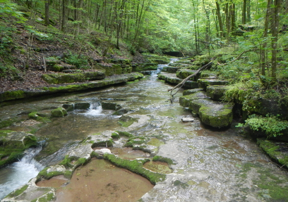
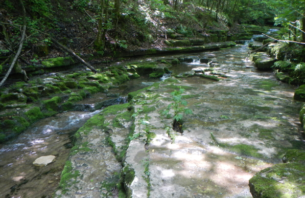
Geomorphological example: Sedimentary basin approaching capacity. Autocompaction or minor erosion slows approach to complete filling. Sediment bypasses the basin during large events, but small events add more material.

2. Increased disturbance frequency.

Force-resistance thresholds may be exceeded due to increased force magnitudes, declining resistance, or a combination. They may also be exceeded due to increased frequency of disturbances (“force events”) that tax the ability of the system to recover to full resistance between events. Thus resistance is more variable and effects become more variable.

Intuitive example: Vegetation community disturbed often, but irregularly, so that succession can never proceed to a late successional community. Thus measurements of, e.g., biomass, NPP, community composition, richness, etc. will be highly variable.

Geomorphological example: A hillslope (e.g., on a lakeshore) that is undercut frequently enough to trigger new mass movements, so that the slope never becomes restabilized. Thu, slope morphology becomes more variable.

3. Rate changes in linked processes. Thresholds may be related to relative rates of linked processes (e.g., glacial accumulation vs. ablation), and could be exceeded due to rate changes in either or both processes. When the linked processes are both changing, but at an unsteady pace or variable rates, the location of the threshold itself may fluctuate, creating variability.

Intuitive example: A bank balance where income is increasing (or decreasing), but at variable pace, and so are expenses. Thus the break-even threshold varies from month to month in an unpredictable way.

Geomorphological example: Both weathering and erosion rates are increased or decreased (e.g., by climate change). However, the relative rates & pace of change vary. Thus the threshold between weathering- and transport-limitation varies, along with denudation rates.

4. Approach to storage capacity.

As storage capacity is approached, additional storage may become more unsteady as the trap or sink becomes less effective. Thus, for instance, small events may continue to add to storage, while large events result in a net decrease in storage.

Intuitive example: Moisture storage in a potted plant. When it is kept near saturation, large events (waterings) mostly splash out or drain right through, while small pourings are absorbed. Measurements of moisture output thus appear to begin “flickering” as the occasional splashouts and drainouts are superimposed on the more regular evapotranspiration losses.

Geomorphological example: A nebkha or field-edge dune begins to approach the maximum height dictated by vegetation. Small wind events add to sand storage in the dune, but large events result in net erosion. Thus measurements of dune sand storage or flux increase in variability.

5. Approach to use or transformation capacity.

Phenomenology similar to item 4 above, but in this case availability of a resource approaches maximum capacity of use by the system. Small inputs can still be fully utilized, but larger inputs cannot.

Intuitive example: Background nutrient levels in an aquatic ecosystem approach the maximum potential rate of uptake. Thus small inputs can be still be processed, but large inputs cannot be fully processed and have toxic effects. Measurements of, e.g., nutrient concentrations & fluxes, dissolved oxygen, community composition, etc. will become more variable.

Geomorphological example: Relatively slow inputs of deposited sediment to soil can be transformed by pedogenesis and incorporated into the soil, resulting in a cumulic (upbuilding) soil. More rapid inputs that exceed the rate of pedogenic transformation bury the soil, and pedogenesis is initiated in the deposited material, resulting in buried soil profiles or bisequal  (or multisequal) soils. If sediment inputs are near the threshold, then small changes in deposition or pedogenesis rates (or small local spatial variations) can lead to divergent pedogenesis.

______________________________________________________________________

Dakos, V., et al., 2013. Flickering as an early warning signal. Theoretical Ecology 6: 309-317.

Kim, D.,  Arthur, M.A. 2014, Changes in community structure and species–landform relationship after repeated fire disturbance in an oak-dominated temperate forest. Ecological Research 29: 661–671.

Kim, D., Shin, Y.H., 2016. Spatial autocorrelation potentially indicates the degree of changes in the predictive power of environmental factors for plant diversity. Ecological Indicators 60: 1130-1141.

Lenton, T.M., 2011. Early warning of climate tipping points. Nature Climate Change 1: 201-209.

Scheffer, M., et al. 2012. Anticipating critical transitions. Science 338: 344-348.

Some miscellaneous observations from the 2016 General Assembly of the European Geosciences Union in Vienna . . . .

Major Concepts = Excellent Session

I participated in a paper session called “Beyond the Case Study: Concepts in Earth Sciences.” Geosciences are of course built on case studies, and without them we would have no useful or interesting theories, hypotheses, syntheses, or conceptual frameworks. But in a professional meeting context you get a bit tired of sitting through the detailed results from yet another watershed monitoring study, lab experiment, numerical model, paleoenvironmental reconstruction or what have you. Unless these things are dead on your own interests, it is much more interesting to be challenged by some big ideas and overarching concepts and themes.

That’s what this session was all about, and it went well. It is rare—in fact I can’t remember the last time—I sat through six presentations in a row that all held my full attention from start to finish.

I wish more scientists would step out with their big ideas, and I hope there are more sessions like this one to encourage that. Take it from me, it doesn’t hurt that much when you get challenged or criticized for them, and you might as well (to strain a baseball metaphor) strike out swinging for the fences as ground out just trying to make contact.

Micha Dietz put together the session, along with Jacky Croke, Maggie Fuchs, and Kevin Norton.

Graph Theory

The only other time I’ve attended EGU was in 2012. At the time I was looking to connect with others applying graph theory in geomorphology, and I only turned up two—Wolfgang Schwanghart and Tobias Heckmann, both from Germany. I met them for lunch, and our jointly authored reviews of graph theory in geomorphology and geosciences arose from that meeting.

Four years later, graphs and networks are all the rage in geomorphology (and other geosciences represented here). It’s great to see how many new applications are being developed, and the potential for so much more. It’s also humbling, as it was the first time I met Wolfgang and Tobias, to see how much better some people are at it than I am.

Connectivity and Tipping Points

Geomorphologists and hydrologists have long been concerned with issues of water and sediment connectivity—whether, how, how much, and how often fluxes occur between various locations and hydrogeomorphic entities. Less than a decade ago, however, connectivity became a major buzzword not just for scientists, but also managers and engineers as a broader community became aware of its importance for issues such as water quality and aquatic and riparian ecology.

This EGU meeting featured an entire day of geomorphological connectivity papers, some of which were simply traditional geomorphic topics packaged as connectivity (after all, what study of mass fluxes and transport does not address connectivity in some fashion?), and some of which addressed emerging issues in connectivity (including application of network and graph theory). Still, one of the principle figures in the rise of the connectivity framework (I won’t mention the name because they didn’t know they might be quoted) indicated that they were getting pretty sick of it all.

Yeah, I understand that. But right now, connectivity sells in terms of grabbing attention, and we should not hesitate to use the term if it fits to get attention. The same goes for Tipping Points. Stuart Lane gave a presentation pointing out (among other things) that the idea of TPs has no “value added” for geomorphology, as everything it includes are already covered, and less ambiguously, by existing concepts.

But tipping point terminology is already out there, prominent in environmental discourse, so why not use it to gain attention, or funding (in conversation later, by the way, Stuart totally agreed)?  Having said that, I presented a poster here on tipping points, am part of a funding proposal under review on the topic, and have previously blogged about it.

At the very least, several of us agreed that someone should start a pub called Tipping Pints. It was funnier if you were there.

To me, colluvium—at least conceptually—is pretty simple. When soil or sediment is eroded (or mobilized via mass wasting) from a hilltop or hillslope, moved downhill, and redeposited before reaching a stream valley, then those deposited materials are colluvium.

But not everyone shares my perspective. Many soil scientists and engineers, for example, restrict colluvium to deposits associated with mass movements. Some geomorphologists attach additional criteria beyond those of my simple definition. This issue is important beyond basic issues of scientific communication, because the identification and measurement of colluvial deposits is critical for studies of sediment budgets and mass balances of hillslopes and drainage basins, and for understanding regolith development and pedogenesis.

Bradley Miller is taking on this terminological, geomorphological, and pedological conundrum (see his blog post on the subject here).  Along with Jerome Juilleret, he has developed an interactive poster that outlines the varied definitions and links you to an online discussion of colluvium definitions. And Miller and Juilleret have developed an online questionnaire on distinguishing between colluvium and alluvium. I took it, and I think you should, too. It is actually fun, at least if you are a geomorphology or soil nerd, and seems well designed to generate some useful perspectives on how geoscientists and environmental scientists perceive and define colluvium. 

No matter what definition you use, identifying & measuring colluvium in the field can be labor-intensive!

From 2010 through the first two-thirds of 2015, at least 211 scientific articles with the term “tipping point” and 109 with “regime shift” in the title were published (according to the Web of Science database, as of 23 November 2015). These span a broad range of science, technology, and engineering, but the geosciences are well represented. In recent years the concept of tipping points in the global environment related to climate change, regime shifts, ecosystem collapse and other phenomena has garnered a great deal of both scientific and public attention. “Tipping point” is often used in public (and sometimes scientific) discourse to refer to impending doom, or at least major environmental changes with uncertain and potentially negative impacts. However, tipping points are not necessarily associated with negative impacts on humans. Nor are they inevitably associated with direct or indirect human agency, as Earth history is marked by numerous tipping points and regime shifts.

Tipping points are a type of threshold phenomenon. In systems theory (and Earth and environmental sciences) a threshold is a boundary separating different behaviors or states (qualitatively different conditions) of a system. Tipping points are thresholds (but not all thresholds are tipping points) that result in rapid or abrupt state changes relative to the time scale under consideration. Regime shifts are threshold-driven state changes that may be gradual or abrupt. Regime shifts are a subset of thresholds that are generally understood to apply at a broad landscape or ecosystem scale.

Understanding scientific concepts is heavily dependent on the metaphors we use to visualize, analyze, and communicate them. Recognizing that tipping point itself is a metaphor, I got to wondering about what other metaphors might be useful in exploring these abrupt shifts in Earth systems.

Balance

The tipping point notion is at least implicitly based on a metaphor analogous to a balance or scale. In fluvial geomorphology this analogy is often used with respect to aggradation or degradation with a diagram or conceptual model like the one below:

www.fgmorph.com/fg_2_9.php

My interpretation of this, by the way, is quite different from the traditional one. Some assume (on the basis of precious little evidence) that fluvial systems seek to equalize sediment supply and transport capacity and keep the scale balanced. My view is that the scale is usually tipped to one side or the other, but increases or decreases in sediment supply or transport capacity can cause it to tip in the other direction.

Seesaw

Since the idea of a balance as a weighing device is indeed to achieve balance, I prefer the seesaw metaphor for the situation described above. This is a pretty good metaphor for a fairly common situation in Earth systems, where an unstable equilibrium separates two alternative stable states.

The Cliff

This analogy is firmly related to a doom-based view of tipping points. The TP occurs when the system is pushed to the edge, and a precipitous decline.

http://livinggreenmag.com/2012/06/13/climate-change/scientists-warn-that-earth-is-close-to-climate-tipping-point/

Dominoes

In this case a line of dominoes is the analog of a complex, interlinked environmental system with many components. Tipping one domino (a local tipping point) will cause some or all of the others to fall as well (a global or regional TP).

http://thedominoeffectmovie.com

Any of these metaphors, and no doubt others, have their advantages in communicating certain ideas and analyzing certain problems. The dominoes analogy seems to me to have particular promise.

Suppose each domino is designated x_i, with i = 1, 2, . . . , n total dominoes. The dominoes are all assumed to be adjacent to at least one other domino. We further assume that a domino tipping either left or right will knock over exactly one other domino (except for the first and last, x₁ and x_n, which could tip in one direction without disturbing other dominoes).

This characterizes (or caricatures) a situation where a local tipping point anywhere is the chain of dominoes has a unique effect. The two end dominoes are all-or-nothing: If they tip one way, nothing else happens. The other way, and every other domino goes down. For all the others, the number of dominoes that fall also depend on which way an individual tips. Using a simple left-to-right description the line of dominoes (i.e., x₁ is the first, left-most and x_n the last, right-most domino), the number of fallen dominoes is n – i + 1 if it tips right, and dominoes x_i through x_n fall. A left tip, and dominoes x₁ through x_i  go over, with the total number tipped equal to i.

Any domino is highly sensitive to any left-tips for of any dominoes to its right, and insensitive to any left-tips to its left, and vice-versa. We can also look at probabilities. If every piece has an equal probability of being disturbed, and falling left or right is equally probable, then p(x_i, R) = p(x_i, L) = 1/2n—that is, the probability of any given domino tipping left or right is 1/2n.

The probability of a tipover at domino j, given the falling or domino i, is as follows:

p(x_j:x_i) = 0 if j > i and i tips left.

p(x_j:x_i) = 0 if j < i and i tips right.

p(x_j:x_i) = 1 if j < i and i tips left.

p(x_j:x_i) = 1 if j < i and i tips right.

This seems to me to convey the idea that tipping points, like pretty much everything else in the geosciences are difficult to generalize about without geographical and historical context!

Axioms of the Dominant Controls Concept

The “dominant processes concept” in hydrological modeling argues, in essence, that there are too many potentially relevant hydrological processes to feasibly or efficiently include them all in a single model. However, in any given watershed a handful of processes dominate the hydrological response, and an effective model may be developed based on those. This argues for adapting models to local conditions and needs, rather than attempting to construct “one size fits all” models designed to handle any watershed, anytime, anywhere. Grayson & Blöschl (2000a) are credited with initiating the DPC; I encountered it through Bellie Sivakumar (2004, 2008).

In an article on avulsions a few years ago, I argued that the dominant processes concept can be generalized to a “dominant controls concept” (DCC) in geomorphology, and probably Earth and environmental sciences more generally. The DCC implies that, while there may exist a very large number of factors and processes that can influence a given phenomenon (in that case, avulsions) in any given geomorphic system some will be irrelevant and others of comparatively negligible influence, leaving a few dominant controls to deal with.

According to the DCC, structure & dynamics of this New Zealand shore platform—like any other Earth surface system—is dominated by a few key controls.

Not long after, I wrote down some axioms of the DCC/DPC, intending to eventually flesh them out in an article.  That looks increasingly unlikely, but as I think they might be useful, I am laying them out here.

The DCC is intended to guide not only predictive modeling, but also any effort to understand, analyze, or represent Earth Surface systems. The axioms:

1. For any Earth surface system (ESS) a few controls account for the great majority of variation. This includes variations in system response and outputs, and also variability of key components and fluxes within the system. My experience with geomorphic, hydrologic, and pedologic systems indicates that the number of dominant controls is generally a half-dozen or less. Note that this refers to specific ESS, such as the Shawnee Run watershed, Kentucky, or the Otter Creek marshes, North Carolina—not to generic ESS such as fluviokarst watersheds or brackish marshes in general.

2. ESS responses to change are dominated by a few critical or essential behaviors or phenomenologies. This is a corollary to axiom 1.

3. Dominant controls & responses vary:                                          

            •Geographically between ESS

            •Synoptically within ESS

            •With spatial & temporal scales.

This axiom recognizes the fundamental, irreducible role of geographical, historical, and scale contingency in ESS—which was the primary motivation for developing the DPC and later the DCC in the first place.

4. Appropriate models or representations include dominant controls and exclude or minimize others. This follows fairly obviously from 1 and 2 above. But since axioms are self-evident truths that require no proof, that’s OK . . . .

5. Appropriate models or representations thus vary geographically, temporally, and with scale.

To me, and I think many others, both personal and collective experience support numbers 1 and 3 above as axiomatic, and if those are accepted, 2, 4, 5 must also be true.

For what it’s worth . . . .

---------------------------------------------------------------------------

Grayson RB, Blöschl G. 2000a. Summary of pattern comparison and concluding remarks. In Spatial Patterns in Catchment Hydrology: Observations and Modeling, Grayson RB, Blöschl G (eds). Cambridge University Press: Cambridge, UK; 355–367.

Sivakumar, B., 2004. Dominant processes concept in hydrology: moving forward. Hydrological Processes 18, 234–235.

Sivakumar, B., 2008. Dominant processes concept, model simplification and classification framework in catchment hydrology. Stochastic Environmental Research and Risk Assessment 22, 737–748.

In my previous post (Soil Erosion Rises Again!) I noted a recent spike in interest in erosion and soil conservation, following previous ones in the 1930s and 1980s. One manifestation is the work of Frans Kwaad, a Dutch physical geographer, who has reinvigorated discussion of the relative onsite and offsite costs of erosion.

Onsite (economic) costs are generally related to declines in crop or grazing productivity, or the loss or degradation of economically productive land. Offsite costs are associated with pollution and infrastructure damage associated with the deposition or delivery of eroded sediment, habitat damage or destruction, nuisance costs of removal of deposited sediment, etc. Kwaad’s work-in-progress synthesizes a number of studies and data sources, and on-balance indicates that off-site costs are greater.

Cleaning up eroded soil after a storm in the Netherlands (F. Kwaad photo).

A key message is that no matter who does the accounting and how they do it, on- and offsite costs of erosion are truly massive, and easily justify any imaginable expenditures on soil conservation, erosion control, and stormwater management.

But, as Kwaad and many of the sources he cites acknowledge, such estimates are problematic. Soil quality is only one of many factors that influences crop productivity, and productivity is only one of several factors that influences monetary values of crops. Similarly, off-site costs of erosion are often entangled with other factors such as, e.g., pesticides, metals and nitrates sorbed to the eroded soil. Second, most of the studies deal with intensive, mechanized agriculture. In such systems, productivity declines associated with reduced soil fertility is often masked with additional inputs of synthetic fertilizers, fossil fuels, and other inputs. There are also many technical issues associated with the monetization of environmental impacts.

Sediment-choked channel during a storm in northern Morocco (F. Kwaad photo).

Maybe most problematically, even if monetization was an exact science, it is only one way of tallying the score, and many would argue that it is not the best or most important. Loss of crop productivity in a subsistence agriculture system, for example, is far more devastating than in industrial agriculture, even though the monetized value may be less. And when ecosystem services, or a favorite fishing spot, are ruined essentially forever, how can you put a value on that?

We live in a society that fetishizes money and numbers, and it is not only inevitable that these will be used to assess impacts, but necessary to address power brokers in language they understand and accept. They key points, to me, are that soil erosion has costs, monetary and otherwise, onsite and offsite. Those costs are fairly easily minimized, as soil conservation and erosion control techniques and technologies are well developed. If monetizing the costs gets attention, and helps justify taking those measures, then so be it. But we should recognize that soil is the natural capital on which the rest of the economy (and most important things) depends!

Soil erosion is a food security issue in India, among other places (http://www.indianbureaucracy.com/loss-of-fertile-soils-a-food-security-…)

In the 1930s, the Dust Bowl and the legacy of massive post-Civil War cut-out-and-get-out logging and, particularly in the south, of what amounts to shifting cultivation brought a soil erosion crisis to the attention of the USA and the world. In the 1980s, a realization that problematic erosion persists despite great improvements in soil conservation and a heightened concerned with nonpoint source pollution from agriculture brought renewed attention to erosion, this time focused particularly on off-site impacts. On-site impacts of soil erosion are the environmental degradation and lost productivity due to soil loss, while off-site impacts are related to pollution and costs associated with where the soil ends up. Now, we are at it again, with another wave of attention to soil erosion.  

Eroded farmland in Alabama, 1930s (WPA photo by Arthur Rothstein).

A recent meta-analysis of global soil erosion rates by a group of Spanish geomorphologists and soil scientists in Geomorphology reveals a surprising amount of variability in measured and estimated erosion rates that has generated a great deal of discussion. And physical geographer Frans Kwaad (University of Amsterdam) has reinvigorated discussion of the relative onsite and offsite impacts of erosion. Finally, loss of peat soils to fire and drainage has led Indonesia to offer a $1 million prize for developing a method to quickly and accurately map the country’s peat soils.

Eroded field in the Netherlands (F. Kwaad photo).

The meta-analysis by Garcia-Ruiz et al. (2015) considered published data from >4000 sites worldwide, finding that “there is extraordinarily high variability in erosion rates, with almost any rate apparently possible irrespective of slope, climate, scale, land use/land cover and other environmental characteristics.” In general, results do not refute the known relationships of water erosion with precipitation, topography, and land use, but the amount of scatter is enormous. More tellingly, Garcia-Ruiz et al. found that apparent rates vary with the method used to measure or estimate soil loss, size of the study area, study duration, and time scale considered. From their abstract:

“ . . . the data suggest that only order of magnitude approximations of erosion rates are possible, and these retain a very large degree of uncertainty. Consequently, for practical purposes such as calculation of global sediment budgets, empirical equations are not a substitute for direct measurements. Our results also show that a large proportion of the experiments have been short-term (less than 3 years), which reduces dramatically the reliability of the estimated erosion rates, given the highly non-normal behavior of soil erosion (time-dependency). Despite the efforts already made, more long-term measurement experiments need to be performed, especially in regions of the world that are under-represented in global datasets.”

Erosion rates vs. annual precipitation. Check out the scatter! Figure from Garcia-Ruiz et al. (2015).

The paper contains the usual call for more data, and the equally usual plea for standardized measurement and reporting procedures. However, in this case there is a better-than-usual case for such calls.

But let me add a few caveats.

First, while Garcia-Ruiz et al. (2015) cast plenty of legitimate doubt on our global-scale understanding of soil erosion rates, that does not necessarily question or invalidate individual studies in context. For instance, you can (and should) question whether erosion-plot results from a cornfield in Ohio measured over two years are comparable to profile truncation estimates covering a 100-year period in North Carolina. But if the studies in question are competently conducted, then you have good data on plot-scale soil loss from a cornfield in a particular 2-year period, and on net soil surface lowering over a century.

Second, don’t let the results make you think we don’t understand erosion causes and processes. We do. There is, of course, always more to be learned, but the basic mechanisms are well understood, and can generally be worked out pretty well for any given situation. The problem is that those situations are extraordinarily variable, and it is thus difficult to generalize from one site to another.

Third, the results underscore the geomorphic folk wisdom that the answer to every question is “it depends on the scale.” With respect to time scales and study durations, we have long known (for a variety of geomorphic processes, not just soil erosion) that longer periods generally yield lower mean rates. This is because the longer the time period, the more likely it is to include periods where nothing much is happening. With respect to area, and spatial scale, it has also been known that soil loss is dominated by hotspots of high erosion, and that within a watershed a small proportion of the drainage area produces a large proportion of the sediment. If you are measuring a hotspot you’ll get high rates, and otherwise you’ll get lower rates. If you sample or measure a large area, the cumulative results will underestimate the hotspots and overestimate the rest. Also, the larger the area the more opportunity there is for temporary storage of eroded sediment, and thus the measurement technique comes into play—measurements of local removal may overestimate the amount of soil leaving the area, while measurements of output from the entire area will underestimate local soil loss.

Finally, uncertainty over quantitative rates of erosion in no way invalidates solid qualitative evidence of erosion problems. If topsoil is removed or thinning, there’s an erosion problem.* If infertile or less fertile subsoils are being exposed, there’s an erosion problem. If eroded sediment is clogging ditches or streams, or piling up along fences or field edges, there’s an erosion problem. If rills appear after a rainstorm, there’s an erosion problem. If you see exposed tree roots or gullies or lag deposits or erosion pavements, there’s an erosion problem. 

No matter what technique you use, or what numbers you get, or how certain you are of those numbers, this area of the Rif Mountains, Morocco, has an erosion problem (F. Kwaad photo).

*”Problem” assumes that the erosion is detrimental to human interests and/or ecosystem services. Certainly erosion occurs naturally, and sometimes with no net adverse impacts. From a purely scientific perspective, you could substitute “accelerated erosion” for “an erosion problem,” with accelerated indicating removal rates well in excess of soil formation or upbuilding rates.

NEXT: onsite vs. offsite costs.

________________________________________________________________________________

Garcia-Ruiz JM, Begueria S, Nadal-Romero E, Gonzalez-Hildago JC, Lana-Renault N, Sanjuan Y. 2015. A meta-analysis of soil erosion rates across the world. Geomorphology 239: 160-173.

The online-first version of an article I co-authored with Chris Van Dyke is now available from Earth Surface Processes and Landforms: “Principles of geomorphic disturbance and recovery in response to storms.”

The abstract:

The most important geomorphic responses to storms are qualitative changes in system state. Minor storms produce no state change or very rapid recovery to pre-storm state, and extinction events wipe out the system. In other cases disturbance results in a state change, which may be transitional (change to a previously existing state), state space expansion (change to a new state), and clock-resetting events that return the system to its initial state. Recovery pathways are much more varied than the monotonic progressions represented in classic vegetation succession and linear channel evolution models. Those linear sequential pathways are only one of several archetypal recovery pathways, which also include binary, convergent, divergent, and more complex networks. Filter dominated systems are more likely to follow linear sequential or convergent patterns, whereas amplifier-dominance is characteristic of divergent and more complex mesh or fully-connected patterns. Amplifier domination is also more likely to lead to evolutionary or state space expansion responses. Amplification and filtering in geomorphic response and recovery can be assessed using the ’Four R’s’ framework of response, resistance, relaxation, and recursion. High resistance and resilience, rapid relaxation times, and stable recursive feedback networks reduce or offset effects of disturbances, thus filtering their impacts. Conversely, low resistance and resilience, slow relaxation, and dynamically unstable feedbacks can exaggerate disturbances, creating disproportionately large and long-lived impacts, thereby amplifying disturbances. Unless new filter mechanisms evolve (either autogenically or anthropically), or the number of extinction or clock-resetting events increases, intensified storminess will result in more geomorphic variability. These ideas are applied to a case study of a flood on the Clark Fork River, Montana, USA.

KEYWORDS: storms; disturbance; recovery; resilience; amplifiers; filters