OK, so I tried to read Salvatore Engel-Di Mauro’s 2014 book, Ecology, Soils, and the Left: An Ecosocial Approach. As a geomorphologist who studies soil erosion (among other things), and as an environmentalist/conservationist interested in the human dimensions of erosion, it seemed a worthwhile piece of work (and probably is).  Years ago I was greatly influenced by Piers Blaikie’s 1985 The Political Economy of Soil Erosion—it even inspired me to develop a (widely ignored and little used, but I tried) method for modeling/estimating soil erosion in less developed countries where technocentric North American and European approaches were unlikely to be applicable.

Blaikie critiqued—often strongly—geomorphologists, soil scientists, and engineers. But he did so without insults and putdowns of scientists and science.

Not so Engel-Di Mauro. A few samples:

Biophysical scientists have proven historically to be largely subservient to the ruling regime of the day (and sometimes emphatically aligned with the ruling classes).

. . . the biophysical sciences are rife with politics, the kind of politics that does not get acknowledged as politics and even somehow passes for objectivity.

Sciences . . . tend to be the sort of capitalism-friendly, classist, patriarchal, Eurocentric, racialized milieu that arguably makes many leftists want to leave or puts them off for good.

A typical pedologist, apparently.

Though Engel-Di Mauro emphasizes a critical approach to the study of scientific practice, the accusations and slurs are presented uncritically, as received truth. He does acknowledge some “good” scientists in an exception-that-proves-the-rule tone, and his criticisms/insults are, no doubt, completely valid with respect to some individuals and institutions. They would be equally true with respect to a number of individuals and institutions in sociology, literature, human geography, economics, art, etc., etc.

But to claim that geomorphologists, soil scentists, ecologists, and biophysical scientists in general and as a rule are racist, sexist, classist tools of the capitalist elite, uncritical, clueless, and completely unaware of any social or political implications of or influences on our work, unless of course we are enthusiastically facilitating capitalist exploitation—well, that’s just crap. I cannot dignify it with any further rebuttal.  

One of the corporate overlords, that we scientists apparently slavishly serve.

But here’s the thing—I’m pretty sure the book has some worthwhile stuff in it. I know I should be a big enough person to overlook the put-downs and focus on the valid bits.

But I’m not.

Partly, I worry that an author who spews such unsupported nonsense (the samples are all from the preface, but there’s lots more where that came from) on one topic might well be doing so on others, where I am not in a position to recognize it as such.

But mainly, it just pisses me off.

Part of what Engel-Di Mauro is doing is trying to convince leftists that it’s OK to care about soil and to (carefully, so as not be tainted by our evil) engage with the biophysical sciences. He probably feels a need to reassure them that he is just as skeptical as they are.

I get that.

But if he wants scientists—the majority of scholars who actually get our hands dirty—to take him seriously, he’s going to have to do better than that, unless most of my colleagues are thicker-skinned and more tolerant of insults than I.

I am not telling you not to read the book, by the way. If you can wade through the evil clueless scientist bunk long enough to get to the good stuff that I reckon is there, by all means do so, and then tell me what it is. 

25 years ago, Vic Baker and Rowl Twidale published an article in Geomorphology called “The Reenchantment of Geomorphology.”  At the time, I found their essay interesting and provocative, but annoying, and I disagreed with much of their message and with their overall tone.  Over the years, however, I have come to have a much different perspective—overall, I have largely come around to Baker and Twidale’s view.

Here’s the abstract of their paper:

Much of modern Geomorphology lacks the enchantment that the science possessed a century ago. Practical and philosophical impediments are thwarting modern attempts to achieve a satisfying understanding of landforms and their genesis. In recent years, even the security of geomorphologists' academic bases has been threatened within the cognate disciplines of Geography and Geology. During the 1960s these fields experienced so-called “scientific revolutions,” which many geomorphologists either uncritically embraced or assumed to be irrelevant. While commendable in spirit, progressive initiatives to establish research traditions in landscape evolution, climatic geomorphology, and process studies all encountered fundamental limitations as unifying themes. More disturbing are ideological impositions that advocate geomorphological concentration on timeless, theoretical, or utilitarian problems. While facilitating precision of explanation and prediction, various geoideological bandwagons may stifle creativity, insight, and intellectual satisfaction. Most insidious is the substitution of elegantly structured methodology and theory for spontaneity, serendipity, and common sense. Hope for the reenchantment of Geomorphology lies in a new connectedness to nature that will facilitate the identification of anomalies and the formulation of outrageous hypotheses of causation. In the words of William Morris Davis, “…violence must be done to many of our accepted principles.” Examples of such ideas may be found in fringe areas of the discipline, including planetary geomorphology, tectonic geomorphology, and denudation chronology with emphasis on ancient paleosurfaces. Geomorphologists should consider inverting their belief that they are achieving progressive (timebound) understanding of invariant (timeless) laws in nature. Rather, they may choose a geophysiological view in which the richness of natural history is revealed in a timeless conversation with the Earth.

 An enchanted venticfact, White Desert, Egyt

Regular readers of this blog (both of you!) may find it surprising that I ever objected to much of this rhetoric, so let me provide a bit of context. I got my PhD in 1985, and most geomorphologists of my generation were trained, even (benignly and informally) indoctrinated, in an approach that eschewed regional and historical approaches (especially Davisian ones!), valorized quantification and modeling, and sought to eliminate geography and history in favor of universal laws. In 1991 I was not only just a few years past this training, but also deep into quantitative models, and had not yet recognized the critical connections between geographical and historical contingency and the complex nonlinear dynamics I was studying. Stuff I wrote in 1992, for example, was concerned with linking nonlinear dynamical systems to the ahistorical approaches of Strahler, Chorley, Leopold, Scheidegger, et al., not to ideas about contingency that I subsequently developed/discovered.

So here come Twidale and Baker, with some critical questioning and sharp critiques of my worldview. At the time I had heard of and read other work by both men, who were then and now widely respected as giants in the field. I had not met either, though I did subsequently, and was fortunate enough to spend several days in the field with Rowl in South Australia in 2005.

In retrospect, I suspect some of my adverse reaction was not just that I disagreed with their take, but because I knew intuitively there was some truth to their critique. And despite my allegiance at the time to a non-reenchantment methodology, their comments about the role of intuition, a sense of wonder, and “conversations with the Earth” resonated with me at some level. Like many of us in the discipline, I got into the study of landforms and surface processes because of a love of and fascination with rivers, beaches, marshes, and such, not due to a fascination with steady-state mass balances, sediment transport equations, or roughness coefficients.

In the past 2.5 decades, I’ve become pretty good at merging my scientist self with the part of me that encounters landforms while holding a fishing rod, a water bottle, a cold beer, or the hand of my wife or child (or, most recently, my granddaughter!). Plenty of encounters with the laser level, soil auger, and other instruments in hand eventually taught me, first, that geography and history always matter, and that we cannot eliminate their influence no matter how much (at least as scientists) we want to. Then I stopped wanting to. One of these days I hope to write a post (or maybe even an article) titled (based on a variation on the subtitle of Stanley Kubrick’s film Dr. Strangelove) called How I Stopped Worrying and Learned to Love Contingency.

Since reenchantment of geomorphology was published, I think a lot more of us have, at least implicitly, come to embrace, or at least accept, Baker and Twidale’s viewpoint. Historical geomorphology is reinvigorated (not least because of new dating methods and technologies), most of us acknowledge (and a significant minority embrace) historical and geographical contingency, and narratives are increasingly valorized by geoscientists rather than being dismissed as “mere” storytelling. On the other hand, a nomothetic, mathematical model-based approach is still dominant, and (too) many of us still fetishize quantification for its own sake.

Anyway, Rowl and Vic, thanks for writing this back in the day! Sorry I didn’t appreciate it then.

In 2012, I published an article in Earth-Science Reviews called Storytelling in Earth sciences: the eight basic plots.  Just for background, the abstract reads thus:

Reporting results and promoting ideas in science in general, and Earth science in particular, is treated here as storytelling. Just as in literature and drama, storytelling in Earth science is characterized by a small number of basic plots. Though the list is not exhaustive, and acknowledging that multiple or hybrid plots and subplots are possible in a single piece, eight standard plots are identified, and examples provided: cause-and-effect, genesis, emergence, destruction, metamorphosis, convergence, divergence, and oscillation. The plots of Earth science stories are not those of literary traditions, nor those of persuasion or moral philosophy, and deserve separate consideration. Earth science plots do not conform those of storytelling more generally, implying that Earth scientists may have fundamentally different motivations than other storytellers, and that the basic plots of Earth Science derive from the characteristics and behaviors of Earth systems. In some cases preference or affinity to different plots results in fundamentally different interpretations and conclusions of the same evidence. In other situations exploration of additional plots could help resolve scientific controversies. Thus explicit acknowledgement of plots can yield direct scientific benefits. Consideration of plots and storytelling devices may also assist in the interpretation of published work, and can help scientists improve their own storytelling.

(Image source: http://www.ntif.org)

In the past few years I’ve gotten a trickle of messages from people interested in the role of storytelling and narrative in geography, geology, and science in general. Sometimes they ask if I’ve published anything else on this topic. The answer is no, but I have blogged previously on the role of metanarratives in geoscience (part 2 here), romantic geomorphology (part 2 here), and the dialectics of geomorphic complexity.

Some correspondents also ask about other literature on this. I am sure there is much more than I am aware of, and the most interesting/relevant pieces that I was aware of ca. 2011 are cited in the storytelling in Earth sciences article. However, I have become aware since of some other interesting work.

Bowman (2001) editorialized in the Journal of Biogeography about the role of environmental history in management of biodiversity. In it, Bowman emphasizes the fact that the popular success of some environmental histories “hinges on the fact that they narrate a compelling story.”

In a piece I should have turned up when working on my article, Norris et al. (2005) developed a theoretical framework for narrative explanation in science. Their focus is on scientific education, but their sophisticated take on narrative structures is applicable to communication among scientists as well.

Daniel Gade’s (2011) book on curiosity and the geographical imagination proposed 14 tenets of the Romantic imagination as it relates to research. Eight of them, in my view, apply readily to geomorphology and geosciences in general, though certainly not all practitioners display or even aspire to all of these traits. The other six can also be interpreted as consistent with and relevant to geoscientists.

In their 2012 piece on “wonder-full geomorphology,” my old pal Deborah Dixon and colleagues wrote of art/geomorphology collaborations, and the role of aesthetics and art in geomorphic science.

Place identities and place attachments (which are closely linked to narratives, stories, and representations) are highly relevant to dealing with climate and environmental change, Devine-Wright (2013) wrote. The research agenda he proposes for investigating and exploiting this fact includes efforts to “capture place attachments and identities,” which obliges engagement with culture, folklore, and arts.

The ethnogeomorphology framework developed by Deirde Wilcock and colleagues (2012; 2013) is multidimensional, but includes a program to integrate environmental stories and narratives with “hard-science” approaches.

My article arose from a sabbatical when I had an opportunity to explore some ideas a bit out of my usual field. I’m sure there is much more that has been done, and to be done, on this. Ideally, I would like to see geoscientists examine their (our) storytelling techniques with the same detail and sophistication we apply to our field, laboratory, and mathematical/statistical methods, and to our cartographical and graphical representations.

_________________________________________

Bowman DMJS. 2001. Future eating and country keeping: what role has environmental history in the management of biodiversity? J. Biogeography 28: 549-564.

Devine-Wright P. 2013. Think global act local? The relevance of place attachments and place identities in a climate changed world. Global Environmental Change 23: 61-69.

Dixon DP, Hawkins H, Straughan ER. 2012. Wonder-full geomorphology: sublime aesthetics and the place of art. Progress in Physical Geography  37: 227-247.

Gade D. 2011. Curiosity, Inquiry, and the Geographical Imagination. Peter Lang Publishers.

Norris SP & 4 others. 2005. A theoretical framework for narrative explanation in science. Science Education 89: 535-563.

Wilcock DA, Brierley GJ. 2012. It’s about time: extending time-space discussion in geography through ‘ethnogeomorphology’ as an education and communication tool. J. Sustainability Educ. 3:

Wilcock DA, Brierley GJ, Howitt R. 2013. Ethnogeomorphology. Progress in Physical Geography 37: 573-600.

Karst development is strongly influenced by climate, both directly (via the moisture balance and temperature regime) and indirectly. The indirect effects include biogeomorphic impacts of biota, and base level changes associated with sea-level and river incision or aggradation. The literature on cave and karst landscape evolution has plenty on the general influence of climate on karstification, the role of base-level changes, and speleothems as proxy records of climate change.  There is little on how (or whether) direct effects of climate change influence the rate or nature of karst development.

One way to approach this would be modeling dissolution kinetics, karst aquifer evolution, and related landscape evolution, by appropriately varying model parameters related to climate. Dreybrodt et al. (2005) give a comprehensive overview of this kind of modeling; while a specific example is Florea (2015), who looked at landscape evolution in epigenic karst aquifers in relation to carbon dynamics. Because other people are much better than I at this sort of thing, I decided to take a different approach, using a qualitative mathematical model of the basic phenomenology and relationships involved in a particular aspect of karst. This sort of reduced-complexity qualitative modeling can be quite useful in some (but certainly not all) geoscience problems.

Karst conduit discharging in Shawnee Run, Kentucky.

Taking the problem of development of a karst conduit (larger conduits may become cave passages), the key “players” are the supply of water to the feature being widened and the evolving conduit, the dissolution processes that enlarge the conduit, the size of the conduit itself, and the velocity of flow. Other things being equal, more water leads to more dissolution, particularly in earlier stages, until the chemical kinetics of dissolution rather than the availability of H₂O becomes limiting. In early stages of conduit development there is often a positive feedback loop where moisture drives dissolution, which enlarges the feature, which allows more moisture, and so on until dissolution becomes rate- rather than moisture-limited or the external supply of water becomes limiting.  At this point conduit size may have little or no influence on moisture supply.

Velocity affects dissolution either positively or negatively. That is, there is a “sweet spot” or an optimum flow rate to maximize dissolution in given conditions. If flow is too fast, there is not enough contact time with the rock. Too slow, and the aggressiveness of the water declines as more and more Ca becomes dissolved. Conduit size (and shape) may positively or negatively influence velocity via the affects on cross-sectional area and hydraulic roughness.  

The qualitative relationships discussed above are shown in the figure below.  

Figure 1

Qualitative systems of this type can be analyzed using qualitative asymptotic stability analysis based on the Routh-Hurwitz criterion, which has been applied in geomorphology, hydrology, pedology, and (especially) ecology. My own description of the method, from way back in the day, is here, but there are many others. If the system is dynamically stable, that suggests convergent evolution and resilience—that is, following a small (sub-catastrophic) change or disturbance, the system can recover toward its previous state. Dynamical instability points to divergent evolution, and effects of changes or perturbations that tend to persist and grow over time.

The system shown above is dynamically unstable. However, though higher dissolution rates increase conduit size, lower rates do not make it smaller again, so in some cases that link could be zero rather than positive. Dissolution is not always moisture-limited, so that link may also be zero. In this case the system is neutrally stable; effects of a change neither grow nor decay over time.  The system can plausibly be dynamically stable if the water supply to dissolution link is zero, and the dissolution to conduit size link is present, but very small and weak compared to other effects in the system. Incidentally, the sign of the two links that may be positive or negative (conduit size-velocity, and velocity-dissolution) does not affect the stability properties.

Karst conduits exposed on the limestone palisades of the Kentucky River, central KY.

So what does this all mean? To some extent it reinforces the idea that earlier moisture-limited stages of conduit evolution are qualitatively different from later, reaction-limited stages. Second, it illustrates that in some systems the irreversible persistence of some changes influences dynamical stability. In this case, once conduits are enlarged, they do not shrink if the processes and relationships that led to their enlargement are changed (at least not due to water flow and dissolution alone; in some cases calcite precipitation, sediment clogging, or mechanical collapse might reduce their size). 

The implications with respect to climate change are that changes in the moisture supply could have significant implications for passages in earlier stages of development, where all links in Figure 1 apply, via the positive feedback loop discussed earlier, which could greatly accelerate conduit development in the case of increasing moisture. However, for the case of decreasing moisture availability, the system may switch into the neutrally stable or stable mode. For a later-stage system where dissolution is reaction-limited, increased moisture would have no significant effect, while a decline in moisture could either have no effect, or trigger a switch to a moisture-limited state. These changes are summarized below:

Now, some caveats:

•This is a highly simplified depiction of karst conduit evolution.

•Other processes—sediment plugging and flushing, Ca precipitation, and mechanical collapse—may influence conduits.

•Conduit development is only one aspect of karst and cave evolution.

•Many factors (particularly biotic and base-level effects) are not considered.

Still, the analysis may provide some useful signposts for further research involving field studies of dissolution processes and cave/karst evolution, and process-based modeling. It also illustrates the fact that when we consider effects of climate on geomorphological (or hydrological, ecological) phenomena, the answer, even with respect to something as broad as stability/instability, is it depends. It depends not just on what type of climate change you are considering, but also on the initial conditions with respect to the state or stage of the geomorphic system in question.

--------------------------------------------------------------------------------------------------

Florea, LJ. 2015. Carbon flux and landscape evolution in epigenic karst aquifers modeled from geochemical mass balance. Earth Surface Processes & Landforms 40: 1072-1087.

Dreybrodt, W., Gabrovsek, F., Romanov, D., 2005. Processes of Speleogenesis: A Modeling Approach. Postojna, Slovenia: Karst Research Institute. 

There sometimes exists an intuitive or cognitive disconnect between the idea that Earth surface systems (ESS) may exhibit divergent evolution associated with dynamical instability and deterministic chaos; and the fact that ESS sometimes evolve so as to increase their complexity and interconnectedness.  Despite the initial apparent inconsistency, these two phenomena can and do happen simultaneously within the same ESS.

Instability/divergence and evolution of increasing complexity are readily reconciled when you realize that instability and chaos are scale-contingent, so that divergence and pseudo-randomness occur within firm limits. Also, these phenomena in effects expand the options an ESS has for its development, thus creating more room for evolution of complexity.

The ecologist Robert Ulanowicz developed the notion of ascendancy as a measure of the complexity and interconnectedness of a system. Ascendancy is influenced by the quantity of matter and energy throughputs, and the network of mass/energy exhanges between system components. Almost 10 years ago (!) I used the notions of ascendancy and Kolmogorov entropy to show how dynamical instability and chaos can increase ascendancy.

This was one of those things that was successful, but not quite enough to justify a publication. Having come back to it now and again over the past decade, I still cannot convince myself there’s enough there for an article. However, I also think it’s too interesting and too good to bury forever.  Thus, I attach here my formal demonstration that instability can lead to increasing ascendancy. It’s in the form of a manuscript with the “theory” section fully developed, but nothing else. 

Geoscientists modeling landscape evolution overwhelmingly (not exclusively, but indeed overwhelmingly) emphasize geophysical aspects, mainly tectonic uplift and erosion. Erosion is typically modeled based on some form of the stream power law, where erosion rates are a power-law function of stream discharge and slope. Discharge is itself often assumed to be a function of drainage area.  There’s nothing wrong with studying the interactions of uplift and denudation without paying much heed to climate, biota, and other factors; I’ve dabbled in this myself.

In a 2009 article, I argued (showed, I like to think) that on a global scale, the biological energy “subsidy” to landscape evolution is comparable to, and even exceeds, the geophysical component. I also introduced a “landscape evolution space” (LES) concept (see also this) attempting to incorporate climatic, biotic, and geophysical contributions. While there is more attention than ever to biotic influences on geomorphology, the LES concept hasn’t gotten much traction, and landscape modeling is still overwhelmingly geophysical. In that’s context, let’s take a look at energy inputs to the Earth’s surface.

The total mechanical power driving global tectonics is 4.8 X 10⁷ watts (W), which translates to 0.297 megajoules (MJ) per square meter per year. By contrast, total solar radiation absorbed the atmosphere and land surface is 240 W m^-2, or 7574 MJ m^-2 yr^-1. On average 5680 MJ m^-2 yr^-1 is absorbed at the surface, and drives biological processes, moisture fluxes, air movements, heat fluxes, etc. (more than 19,000 times the tectonic power). Global mean gross primary productivity (energy used to produce biomass, plus respiration) is estimated at 315 to 420 MJ m^-2 yr^-1.

The mean elevation of the continents is 874 m. Given the density of crustal rocks, the potential energy associated with moving all mass above sea level to below base level averages 22.698 MJ m^-2 . Even if this were entirely accomplished in a century, the rate of potential energy conversion would be only 0.227 MJ m^-2 yr^-1; 2.27 X 10^-5 if we give it a million years, which is still unrealistically fast.

Before any of that mass can be moved, however, it must be converted to transportable material. Estimating the energy required to break down rock is fiendishly difficult, but in the past I’ve used tensile strength (resistance to a force tending to tear a mass apart) as a rough index. Typical tensile strength of rocks ranges from about 4 to 30 megapascals (MPa = 1 MJ m^-3). With a mean of 847 m³ of rock per m² of the land surface, this implies about 3500 to 26,220 MJ m^-2 to get the job done. In the unlikely event it all got done in a century, we’re talking 35 to 262 MJ m^-2 yr^-1. If we give it a million years, then 0.026 to 0.0045 MJ m^-2 yr^-1. Of course, that’s assuming that a cumulative energy input can eventually add up to the threshold tensile strength; we don’t really know if that’s true.

A graphical comparison looks like this:

Energy inputs associated with total solar radiation absorption, ground absorption, gross primary productivity, tectonics, rock breakdown, and potential energy (PE) conversion rates associated with reducing continents to sea level. The breakdown and PE figures assume that this is accomplished within 1 Ma, an unrealistically rapid rate.

But wait—the graphic above has a logarithmic scale; otherwise the last four would not be discernible. Below is the same figure with an arithmetic scale, showing that even though the tectonic power is an order of magnitude or more greater than the (unrealistically high) breakdown and PE rates, it is still invisible compared to the solar and biological inputs.

So what does all this mean? First, some caveats—these are rough, back-of-the-envelope calculations based on global estimates of processes that vary wildly geographically and temporally. But still, allowing for error and variability, the implications are pretty clear:

•Solar and biological energy inputs to Earth surface systems are far higher than any energy associated with tectonics or mechanics of mass transfers. Even if only a microscopic fraction of this solar and biological input is geomorphologically significant, it is still a helluva lot!

•Energy inputs required to break down rock  are (at least) two to three orders of magnitude higher than the rate of potential energy conversion associated with moving mass to base-level.

•Energy inputs of tectonic uplift are, globally, more than sufficient to “replenish” losses from denudation.

The basis for the quantitative estimates above comes from:

Phillips, J.D. 2009. Biological energy in landscape evolution.  American Journal of Science  309: 271-290.

Smil, V. 2008. Energy in Nature and Society. MIT Press. 

More shameless self-promotion: The online first version of my new article in Progress in Physical Geography is now available: Biogeomorphology and Contingent Ecosystem Engineering in Karst Landscapes. It is not uncommon to acknowledge anonymous reviewers in an article, and I do so here, but it does not do justice to the breadth, depth, and insight of comments I received on an earlier version from three reviewers (which ran to 14 pages!). Whatever the flaws of the final product, it is a heck of a lot better as a consequence of their efforts. Thanks, whoever you are!

When we (scientists) talk and write about complexity in recent years, the focus is on complex nonlinear dynamics, and related phenomena such as deterministic chaos, dynamical instability, some forms of self-organization, fractal geometry, etc.  These are forms or sources of complexity that are intrinsic to the structure of dynamical systems, but these are hardly the only things that make systems complex. So, to make sure we don’t forget the elements of complexity that transcend so-called “complexity science,” I present the Top 10 Forms of Complexity in Earth Surface Systems (ESS). ESS is a blanket term that includes geomorphic systems, landscapes, ecosystems, soil systems, etc.  Even though the items are numbered, they are actually in no particular order. Many ESS may exhibit only a few of these forms, and still be quite complex!

The list I was gonna do has already been done (http://grogsmovieblogs.com/). 

Forms of Complexity in Earth Surface Systems

1. Number of components.  Earth surface systems may have a very high number of components (landforms, soils, chemical components, organisms, species, microclimates, etc.).

2. Degrees of freedom. The large number of components and dense network of connections and relationships between them means that ESS have many different ways or modes of responding to change, and multiple alternative configurations for a given set of boundary conditions.

3. Mutual adjustments.  Due to feedback relationships, ESS components often feature mutual adjustments, whereby components both affect, and are affected by, each other.

4. Changing interconnections. The existence or presence, rates, and intensities of interconnections and feedbacks change. The components are also dynamic.

5. Multiple Scale Causality.  ESS phenomena are not controlled primarily by either bottom-up (microscale to macroscale) or top-down causality. Rather they are determined by multiple processes and controls acting at a range of spatial and temporal scales both larger and smaller.

6. Variability I.  Extrinsic factors that influence ESS are strongly heterogeneous in space and time.

7. Variability II. ESS themselves are strongly heterogeneous in space and time.

8. Nonequilibrium.  ESS are often in states not in, near, or approaching steady-state, thermodynamic equilibrium, or other equilibria.

9. Historical contingency. The direction and magnitude of change is influenced by pre-existing conditions and past events. ESS development is path-dependent.

10. Nonlinearity.  ESS are nonlinear, which enables the possibility of complex phenomena such as dynamical instability and deterministic chaos. 

Hot off the press--more fun with graph theory!

Phillips, J.D. 2016. Identifying sources of soil landscape complexity with spatial adjacency graphs. Geoderma 267: 58-64.

Abstract: Soil landscapes often exhibit complex spatial patterns, with some aspects of soil variation apparently unrelated to measurable variations in environmental controls. However, these local, contingent complexities are not truly random or intrinsically unknowable. The purpose of this work is to develop and apply a method for identifying or teasing out causes of soil landscape complexity. Soil spatial adjacency graphs (SAG) represent the geography of soil landscapes as a network that can be analyzed using algebraic graph theory. These SAGs include linear sequential subgraphs that represent sequences of soil forming factors. The number and length of these soil factor sequences (SFS), and their associated spectral radius values, determine whether the SFS are sufficient to explain the spatial pattern of soil adjacency. SAGs and associated graph theory methods provide useful tools for guiding pedological investigations and identifying gaps in knowledge. The methods also allow sources of soil landscape complexity and variability to be determined in a way that can help assess the underlying deterministic sources of chaos and dynamical instability in pedology. The approach is applied to a soil landscape in central Kentucky, producing a SAG with 13 nodes (soil types) and 36 links indicating whether the soils occur contiguously. Five SFS were identified, the sum of whose spectral radius values is 6.35. The spectral radius of the SAG is 6.56, indicating that the SFS can explain most, but not all, of the complexity of the soil relationships. The analysis also points to potential environmental controls that could potentially enable full explanation. 

In many of my writings I advocate an alternative to reductionist approaches to science. By alternative, I mean a complementary, different way of doing things, not a replacement for reductionism. Many excellent reviews of scientific approaches, viewpoints, and methodological stances exist by historians, philosophers and sociologists of science, and by scientists themselves. I do not intend to review or critique these various approaches here. Further, I have no intent to deny the value or necessity of reductionist science. The crux of my argument is that a reductionist approach, by itself, is inadequate or incomplete for understanding Earth.

The American Heritage Dictionary defines reductionism as an attempt or tendency to explain a complex set of facts, entities, phenomena, or structures by another, simpler set, and provides a quote from John Holland:

For the last 400 years science has advanced by reductionism ... The idea is that you could understand the world, all of nature, by examining smaller and smaller pieces of it. When assembled, the small pieces would explain the whole.

We can distinguish between the practice of reductionist science, pursuing understanding and meaning using the atomistic tools of reductionism, versus a stronger philosophical/theoretical stance. The latter holds that complex systems or ideas can always be reduced to a set of simpler, more fundamental components, and that fundamental or first principles always reside at the smallest level. A belief that reductionism is the primary and preferred path to scientific explanation is by no means rare among scientists, but is less prevalent than a simple acceptance of reductionism as a valid methodology or tool. For instance, the population of biologists using reductionist methods is much larger than the population of biologists who believe that all biological phenomena can ultimately be explained by mechanisms operating at the molecular (or smaller) level.

I am arguing, then, not against reductionism as a valid and useful methodology. In fact, I would argue that it is, and always will be, necessary. I do contend that reductionism by itself can never fully explain Earth surface systems, that reductionism is often not be best approach for some problems, and that where alternatives exists, reductionist methods and interpretation are not necessarily superior or preferable. Why not?

Multiple Scale Causality

In the experimental and laboratory sciences, observed patterns and processes can sometimes be conceptualized straightforwardly as macroscale manifestations of microscale processes. In field-based sciences, however, it is more typical that observed patterns or system states are attributable to multiple processes and controls. Further, those multiple controls operate at multiple spatial and temporal scales--both larger and smaller than the scale of observation.

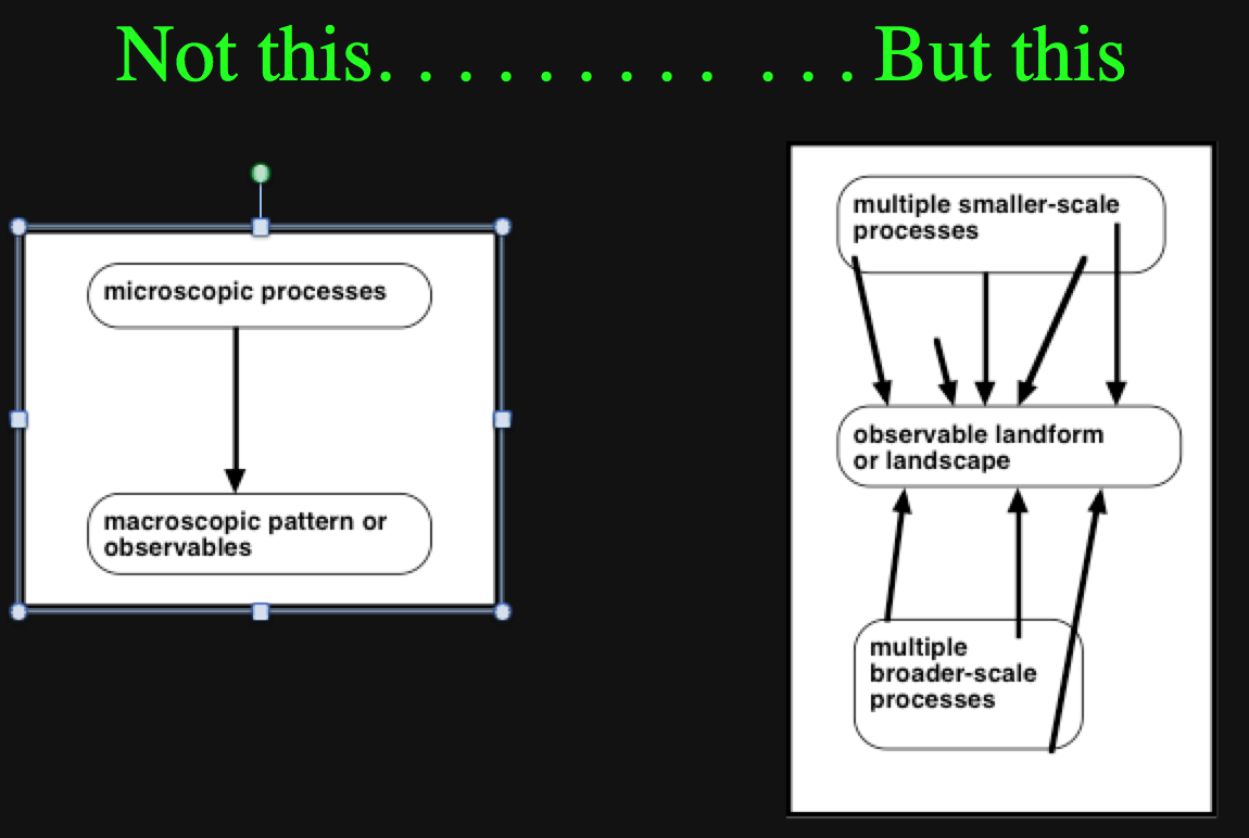
Landforms are a good example. They are created by a number of processes acting at molecular and granular scales (e.g., biological and chemical weathering, erosion, and sediment transport), by factors operating over much broader scales (climate, tectonics), and by controls such as geological structure, which may operate at scales ranging from granular to continental. This notion of multiple scale causality (MSC) not only recognizes multiple processes and controls acting at a range of scales, but also recognizes (in contrast to a strict reductionist approach) that the relevant ‘‘first principles’’ may operate at levels other than the smallest microscales.

Even among Earth and environmental scientists acknowledgement of MSC is not universal, and some emphasize causality at single, particular scales. However, such emphasis does not necessarily imply the rejection of causality at other levels. The evolutionary ecologist, for instance, does not necessarily deny the importance of microscale processes even as she focuses on macroscale evolutionary phenomena. Similarly, the dynamic climatologist, concerned chiefly with atmospheric physics, is unlikely to reject the relevance of synoptic climatology. Recognition of MSC is often implicit: though particular causal agents and scales may be emphasized, causality at other scales is at least indirectly acknowledged. Accordingly, despite the tradition of reductionism, in the field-based sciences claims of causality residing entirely at a given scale are rare.

Ideally, we directly confront MSC, by deliberate attempts to minimize effects at some scales and maximize effects of others, or by isolating scale-contingent causes and explanations. Even when MSC is explicitly recognized, we often seek causal explanation or representation (cartographic, mathematical, conceptual, epistemological, or otherwise) that can accommodate the vast range of potentially relevant scales. Such representations can be reductionist, as in attempts to understand climate on the basis of the fundamental equations of motion or landscape evolution in terms of microscale process mechanics. But reductionists have not cornered the market for attempts at seamless cross-scale representations. Certain complex systems theories have been proposed as covering laws or metaprinciples for geomorphology, biogeography, biodiversity, and evolution; or even nature in general.

On the other hand, some (including myself) maintain that fundamental changes in controls over process-response relationships occur as spatial and temporal scales change, and that unitary, seamless explanation across scales is not only difficult, but fundamentally impossible or unfeasible.

One approach to MSC is via study design. Some are specifically geared toward minimizing—ideally, eliminating—the influence of all but one or a handful of controls or variables. In other cases, investigators simply narrow the focus to minimize variability in broader-scale factors or expand the focus in the sometimes realistic hope that local-scale variations will cancel each other out or be obscured by broader scale factors. Another strategy for coping with MSC involves analytical methods to disentangle the explanatory contributions of variables operating at a range of scales, or at least isolate the variance contribution of a particular scale of interest.

Eco- and geoscientists sometimes cope with MSC, especially in practical applications, by acknowledging that variability is influenced by multiple sources and is manifested at a variety of scales, and then seeking to identify the dominant or critical scales in the context of a particular problem. Geostatistical analysis, for example, is often aimed at identifying the area or distance over which spatial variables are dependent or independent. Other approaches seek to determine the resolution or scale at which variance of the phenomenon of interest is minimized—e.g., determination of representative elementary areas and volumes in hydrology.

An explicit approach to MSC that has been applied in ecology, biogeography, geomorphology, and other fields is hierarchy theory. The fundamental idea is that a hierarchy of spatial scales is identified. In this hierarchy, at any given level of i, there exist controls or influences operating at adjacent larger and smaller scales, i -1, and  i + 1, which may be observed at, and are relevant to, level i. Processes at levels further removed, at either broader or finer scales, operate either too rapidly and finely, or too slowly and broadly, to be observed or manifested at i. Ideally, these hierarchies  allow functional relationships to be transferred up and down the scale hierarchy.

Other, analytically explicit, efforts to engage MSC, include local forms of spatial analysis and entropy decomposition. These generally deal with the issue of assessing the contribution of global and local factors (defined broadly) to the structure and/or variability of spatial patterns.

Independently of formalisms such as hierarchy theory and MSC, defining geographical regions—ecoregions, biomes, agricultural regions, physiographic provinces, etc.--is based on attempts to separate groups of local-scale (within regions) and broader-scale (between regions) controls. In other words, regional delineations attempt to minimize within-region (and maximize between-region) variations.

Fundamentally, however, the basic point is this: Real-world Earth surface systems are characterized by multiple scale causality, reductionist approaches alone are not sufficient for fully understanding them. The other side of the coin is that methods that deal with the most atomistic scales—reductionist methods—are necessary for understanding them.

All Other Things Are Never Equal

Basic two-way, cause-and-effect relationships in the sciences are generally based on the principle of ceteris peribus—all other things being equal (AOTBE). For example, AOTBE, increasing CO₂ concentrations in the atmosphere have a fertilization effect, increasing plant productivity. Of course, plants ability to use the additional CO₂ depends on their having adequate supplies of sunlight, water, and nutrients. As greater atmospheric CO₂ influences climatic variables that in turn influence plant growth, and the activities that change atmospheric chemistry also modify nutrients and other edaphic factors, all other things are not equal. In ESS, all other things are never equal. Why? Because everything is connected to everything else. This maxim has been cited as the First Law of Ecology, the First Law of Environmental science, and the First Law of Geography.

Everything is not literally related to everything else in the sense of direct, tracable, causal, significant links between any two objects, processes, systems, or places. But everything is related to everything else in the sense that Earth system are characterized by multiple, interrelated components and controls. Our world is seen and analyzed by geoscientists and ecoscientists in terms of maps, webs, matrices, flow charts, multiple equation systems, and other representations of multiple, interconnected, mutually adjusting objects or phenomena. Places and environmental systems are understood as the outcome of multiple, interrelated forcings and controls and complex histories.

All humans (or other species), for instance, share common genetic ancestors, and all of us play our roles in the carbon/oxygen cycle with every breath we take, alongside other processes and entities, animate and inanimate. Additionally, long-range interrelationships and teleconnections are typical of ESS: Sea surface temperature anomalies in the equatorial Pacific or the North Atlantic have climatic and oceanographic repercussions around the globe. Commodity price changes in China or Chicago affect land use, soil erosion, and nutrient budgets on fields and paddocks around the world. Coastal landforms in British Columbia or Sumatra may be linked to long-ago, far-away, undersea earthquakes or landslides that triggered tsunamis.

Bailey, Bones & Butterflies

More than a decade ago, writing along these lines, I spoke of the vast web of connections using the metaphors of Bailey effects, bones, and butterfly effects. The “George Bailey Effect” is named after the protagonist of Frank Capra’s 1946 film ‘‘It’s a Wonderful Life,’’ based on a story by Philip Van Doren Stern. George Bailey suffers a run of terrible luck and self-doubt. In despair and attempting suicide in the belief that his life has not been productive or worthwhile, Bailey is rescued by a guardian angel. He is shown an alternative reality; what his community would be like if he had never been born—in the story, a much more desperate, depraved, and depressing place, because the good but relatively routine acts of kindness, bravery and common sense George Bailey committed had not happened. The message: apparently minor actions of an individual may have ripple effects and chain reactions that produce dramatically different outcomes.

Bailey Effects are based on conditionality. Whether or not George saves his brother Harry from falling through the ice as a child, determines whether a loaded troop ship is, or is not, saved by the heroic actions of Harry Bailey later on. The conditionality type of contingent connectedness is common in nature. For example, if the surface cold air layer in a winter inversion is shallow rather than deep, then the precipitation is freezing rain instead of sleet. The freezing rain may in turn result in an ice storm, the effects of which then influence forest species composition (Lafon et al. 1999). Many ESS are conditional with respect to the occurrence, frequency, and timing of factors such as storms, fire, sea surface temperature anomalies, or inherited effects of landform singularities.

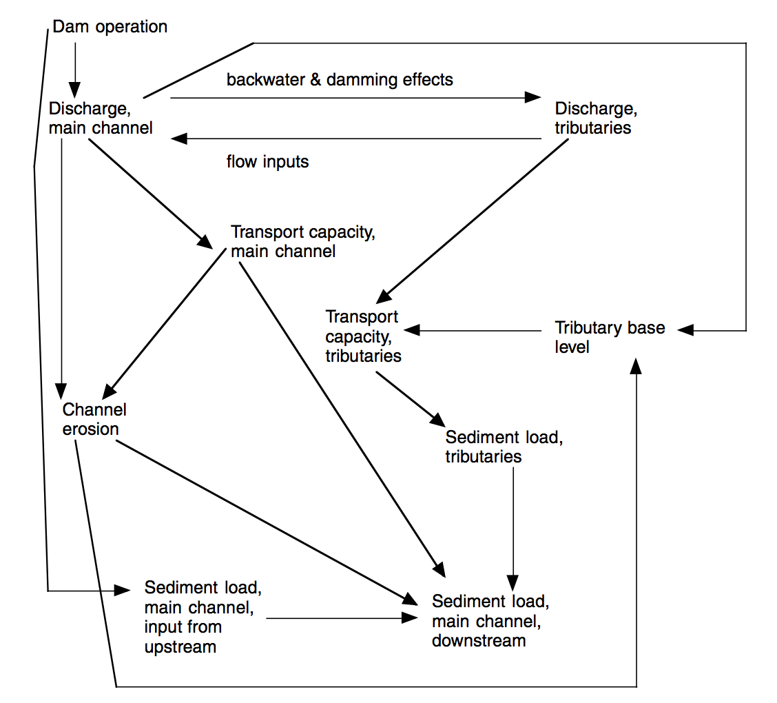
Complex interrelationships between key geomorphological factors downstream of a dam (Figure 2 from Phillips, J.D. 2003.  Toledo Bend Reservoir and geomorphic response in the lower Sabine River.  River Research and Applications  19: 137-159).

The ‘‘bones’’ connections indicate physical, mechanistic, causal interconnectedness, based on the metaphor of a skeleton: the foot bone’s connected to the ankle bone, the ankle bone’s connected to the leg bone, etc.  “Bones” connectivity may be long and complicated, but the chain of interrelationships is clear. This type of relatedness is also common in ESS, and arises mainly due to the presence of numerous components or degrees of freedom, hooked together in long, interconnected chains of causality. Visual evidence is apparent in any detailed diagram of  the carbon or nitrogen cycle, a watershed system, an ecosytem, marine food web, etc.

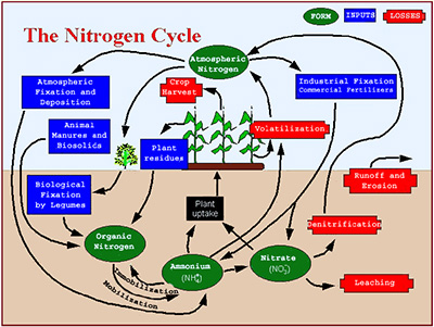
Nitrogen cycle in soils--simplified! (http://www.extension.umn.edu).

“Butterflies” refers to the famous butterfly effect metaphor from chaos theory. A presentation at a scientific meeting by Edward Lorenz in 1972 was titled ‘‘Does the flap of a butterfly’s wings in Brazil set off a tornado in Texas?’’ This was based on Lorenz’s now-famous early work on chaotic dynamics in the atmosphere, where he showed the fundamental equations of motion to be highly sensitive to initial conditions. This sensitivity and chaotic divergence over time gave rise to the notion that a tiny change at a given place and time—e.g., the flap of a butterfly’s wing—might lead to disproportionately large results, far away. Thus ‘‘the butterfly effect,’’ one of the favorite metaphors of chaos and complexity theory. As an aside, as far as I know, no one has ever followed up on my suggestion that “an interesting exercise in trivial geography and chaos theory would be to catalog citations of the butterfly effect, with a map of the different locations of the butterfly and the storm.”

Many environmental systems are, or can be, deterministically chaotic. This means that the effects of minor variations in initial conditions, or of small perturbations, are exponentially magnified over time. Butterfly effects imply elaborations of both Bailey Effects and ‘‘bones’’ connections. Chaos (= dynamical instability) produces the possibility of Bailey effects disproportionately large and long-lived relative to the initial stimulus, and causal webs more subtle and complex than leg bones connected to knee bones connected to thigh bones suggests. Butterfly effects also make possible historical connectedness via ‘‘memory,’’ in the sense that the effects of variations or disturbances that are no longer detectable are manifest in the current state of the system.