Scientists, including geographers and geoscientists, are easily seduced by repeated forms and patterns in nature. This is not surprising, as our mission is to detect and explain patterns in nature, ideally arising from some unifying underlying law or principle. Further, in the case of geography and Earth sciences, spatial patterns and form-process relationships are paramount.

Unfortunately, the recurrence of similar shapes, forms, or patterns may not tell us much. Over the years we have made much of, e.g. logarithmic spirals, Fibonacci sequences, fractal geometry, and power-law distributions—all of which recur in numerous phenomena—only to learn that they don’t necessarily tell us anything, other than that several different phenomena or causes can lead to the same form or pattern. The phenomenon whereby different processes, causes, or histories can lead to similar outcomes is called equifinality.

Center pivot irrigation in Kansas, USA (USGS photo).

To illustrate, let’s use an example of a shape that occurs commonly in nature—the circle (and its 3-D relative, spheres)—but that we haven’t tried to ascribe to some fundamental overriding or underlying law of nature (at least not in recent decades).

In the landscape circular shapes are everywhere—animal burrow openings, center-pivot irrigation areas, impact craters (from raindrops to meteors), explosion craters, sinkholes, weathering cavities, tree canopy “footprints” (driplines).

Sinkhole near Mellrichstadt, Bavaria, Germany (photo: Wikimedia Commons).

The simplest answer is that circles and spheres are efficient. The circle is the 2D shape with the smallest perimeter/area ratio, and the sphere is the most efficient 3D shape for enclosing a given volume. Thus an ant or a wombat digging a nest or burrow seeking to get the job done with least effort constructs a more or less circular opening. Surface tension acting to pull molecules into the tightest possible grouping forms spheres, and thus the effects of these spheres (bubbles) tends to be approximately circular or half-spherical (e.g., cavitation pits in rock). Farmers seeking to irrigate the maximum area of cropland with the minimum amount of pipe use the center-pivot system where topography allows it, resulting in circular vegetation and soil moisture patterns.

So are all landscape circles a manifestation of geometric efficiency? Not quite.

Lunar craters (NASA photo)

A point-centered disturbance with no directional bias (that is, no tendency for effects to be significantly greater in any particular direction away from the point) also produces a circle. Thus explosion craters from volcanoes or bombs, and impact craters are approximately circular. So too for sinkholes formed by solution centered on a vertical joint.

Isotropic dispersion from a point also produces circular patterns. When not affected by other plants or structures, tree branches grow away from the trunk with an equal probability in any direction (same for roots below the ground for trees with lateral roots). Over time the extent of branches and foliage away from the trunk is approximately equal on all sides, so that the zone of influence on the ground reflected by driplines, litter fall, and soil moisture drawdown is circular. Animals foraging from a central point (nest or burrow) will also produce circular impact areas when resource distribution in isotropic.

Tree canopy dripline (durianinfo.blogspot.com)

In the atmosphere the combination of the pressure gradient force and the Coriolis effect produce circular flow around a low pressure center (or a spiral into the low near the ground, where friction plays a role). Thus produces circular patterns of wind and clouds in cyclonic storms.

Typhoon Maysak as seen from the International Space Station (www.abc.net.au).

Finally, there is preferential preservation. In some cases the processes that produce a given form may not necessarily tend toward maximum efficiency, but once formed, those more stable or efficient structures may be preferentially preserved. Thus, for example, weathering cavities on a rock surface with a more spherical (or hemispherical) shape may be more mechanically stable and thus preferentially preserved compared to other cavity shapes of similar volume.

Weathering cavities, Kaikoura Peninsula, NZ (Stefanie Boltersdorf photo) 

Circular and spherical features are therefore examples of equifinality. Even though the explanations above could perhaps be lumped together into two general categories of efficiency-based explanations and point-centered processes, no single explanation applies to all circular or spherical features. In this the circle is no different than a number of other shapes, patterns, and distributions found in nature. 

Some comments from a reviewer on a recent manuscript of mine dealing with responses to disturbance in geomorphology got me to thinking about the concept of disturbance in the environmental sciences. Though the paper is a geomorphology paper (hopefully to be) in a geomorphology journal, the referee insisted that I should be citing some of the “foundational” ecological papers on disturbance. These, according to the referee, turned out to be papers from the 1980s and 1990s that are widely cited in the aquatic ecology and stream restoration literature, but are hardly foundational in general.

Consideration of the role of disturbance goes back to the earliest days of ecology, and is a major theme in the classic papers of, e.g., Warming, Cowles, and Clements in the late 19^th and early 20^th centuries. A general reconsideration (“reimagining” is the term many would use, but I’ve grown to hate that overused word) of the role of disturbance in ecological systems was well underway by the 1970s, and the last five years or so have seem some very interesting syntheses of these emerging ideas (two I especially like are Mori, 2011 and Pulsford et al., 2014).

Geomorphic disturbance in Cameron Parish, Louisiana: washover, beach and dune erosion, and barrier breaching following Hurricane Rita, 2005 (Google Earth^TM image).

Disturbance has also been a venerable topic and concept in geomorphology, though it often goes by other names (perturbations, cataclysms, castastrophic events, forcings, environmental change, etc.). One reason for this is that the time scale relevant to ecological disturbances is commensurate with the time scale of organisms (a century or less for most). Geomorphic disturbances include this time scale, but also much longer, geological, time periods. The very perception or identification of disturbances depends on the time scale—a glacial advance, for example, may be a persistent environmental change at one time scale and a system perturbation at another. An uprooted tree may be a significant perturbation at a relatively small spatial and temporal scale, but insignificant at much broader scales.

A geomorphological, ecological, and pedological disturbance—tree uprooted by a 2007 windstorm in the Czech Republic.

The consideration of the role of disturbances at an “ecological” time scale in geomorphology goes back at least as far as in ecology itself—Nathaniel Shaler (1888) wrote about soil disturbances by fauna. In recent decades much of the literature on disturbance in geomorphology in couched in terms of the concept of landscape sensitivity (e.g.,  Brunsden and Thornes, 1979; Thomas and Allison, 1993; Thomas, 2001).

The surge of interest in biogeomorphology recently has resulted in a mixing of geomorphic and ecological concepts of disturbance, and that’s not a bad thing. We just have to keep in mind that geomorphology has developed disturbance-related concepts independently of ecology, and that if you want to consult truly “foundational” work, you’ve got to go back a century or more.

Brunsden D, Thornes JB. 1979. Landscape sensitivity and change. Transactions of the Institute of British Geographers 4: 463-484.

Mori AS. 2011. Ecosystem management based on natural disturbances: hierarchical context and non-equilibrium paradigm. Journal of Applied Ecology 48: 280-292.

Pulsford SA, Lindenmayer DB, Driscoll DA. 2014. A succession of theories: purging redundancy from disturbance theory. Biological Reviews doi: 10.1111/brv.12163.

Shaler NS. 1888. Animal agency in soil-making. Popular Science Monthly 32: 484-487.

Thomas DSG, Allison RJ (editors). 1993. Landscape Sensitivity. British Geomorphological Research Group, 359 p.

Thomas MF. 2001. Landscape sensitivity in space and time—an introduction. Catena 42: 83-98 (introduction to special issue). 

Fluvial geomorphologists, along with hydrologists and river engineers, have long been concerned with the flows or discharges that are primarily responsible for forming and shaping river channels. In the mid-20^th century it was suggested that this flow is associated with bankfull stage—the stage right at the threshold of overflowing the channel—and that this occurs, on average, about every year or two in humid-climate perennial streams. If you have to choose just one flow to fixate on—and sometimes you do, for various management, design, and assessment purposes—and have no other a priori information about the river, bankfull is indeed the best choice. But, of course, nature is not that simple.

Some streams have more than one (range of) discharge(s) that are critical in forming or maintaining the channel. Some channels and some discharge regimes are in the process of changing or adjusting to new environmental constraints, such that the whole idea of a single formative discharge is a moving target. Some streams undergo cycles—or perhaps episodes is a better word—of channel infilling and excavation. Sometimes, even within humid temperate climates, the bankfull flow does not correspond with a 1- to 2-year recurrence interval. And where it does, it is typically so only when you calculate it using the annual maximum discharge, not using partial duration, daily, or other series.

Banks of the Kentucky River

Without even going into streams in other climate regimes, or bank geometry that makes it difficult in some cases to define exactly where the bank tops are, you have compound channels.  Here major incision events or episodes create a large macrochannel, with inset floodplains or benches defining a smaller channel within (no doubt there other scenarios for compound channels, too).

The relationship between bankfull flow and the year-or-two mean recurrence interval has become so entrenched that there exist techniques designed to identify a “bankfull” level within incised channels where the expected recurrence interval discharge does not correspond with the bank tops (incidentally, that’s why I use the term banktop flow to avoid confusion).

Anyway, a couple years ago I did a study looking at threshold discharges along a 681 km reach of the lower Brazos River, Texas, for thalweg connectivity (to maintain continuous downstream flow), bed inundation (the entire river bed is inundated), high but sub-banktop flows, channel-floodplain connectivity stages (where water is exchanged between the channel and floodplain, and overbank flow. I also estimated thresholds for transport of sand bed forms and medium gravel, and for cohesive bank erosion. The article based on that study just came out in Hydrological Sciences Journal.

I’ve pasted in the abstract below, but the headline is that no single flow is dominant either hydrologically or geomorphically, and the one to two-year flood has no special significance. Also, due to backwater flooding of tributaries, high-water subchannels that are activated by sub-banktop stages, and occasional gaps in the natural levee, channel-floodplain connectivity occurs at much lower discharges than overbank flooding.

I know from my own studies and experience that these phenomena also occur in other rivers of the region, and from the literature that there are many streams where no single flow is dominant. It will be interesting to see where future studies of reference, critical, threshold, or channel-forming flows take us.

One of the classic principles/relationships in biogeography is called the species-area curve, relating the number of different species found (usually of some particular taxonomic group; e.g., birds or plants) to the area sampled. These curves are usually well fit by an exponential relationship:

S = c A ^b

where S is the number of species, A is area, c is a constant representing the number of species in the smallest area sampled, and b represents the rate of increase of species with area. While b could be greater than 1 if major biogeographical boundaries are transgressed (so that whole new sets of species are encountered), otherwise b < 1, and usually much less; 0.25 is a fairly common value.

Juanjo Ibanez and I (in separate studies) found that similar trends apply to soil diversity, with S in this case indicating number of different soil types (e.g., soil series). In his very broad scale analyses, Juanjo also found b » 0.25, while in my landscape-scale studies b was in the range of 0.6.  Syntheses of this work are found in the book Pedodiversity (CRC Press, 2013) edited by Ibanez and James Bockheim.

The flattening out of the curves (i.e., b < 1) reflects the fact that as more area is sampled, you do find new soils or species, but increasingly you encounter types that have already been enumerated. Does the same general pattern hold for diversity of geomorphology along rivers?

I have done geomorphic zonation studies for four different rivers in Texas in support of the Texas Instream Flow Program, along lengths of river ranging from about 210 to 700 km (Sabine, Trinity, Brazos, and Guadalupe Rivers). From this, a relationship between river or valley length sampled and geomorphic diversity can be determined.

The geomorphic zones were identified using the River Styles approach pioneered by Kirstie Fryirs and Gary Brierley (see their book Geomorphology and River Management. Applications of the River Styles Framework, Oxford UP, 2005). Geomorphic zones or river styles were identified based on similarities of geological setting, hydrologic regime, valley confinement, dominant substrate types, morphometric properties such as slope and sinuosity, planform, and other properties relevant to specific rivers such as presence or absence of sandy point bars, avulsed reaches, and dam effects.

Using these maps, for each river I sampled every 10 km in the upstream-downstream direction, counting the total number of geomorphic zones or river styles encountered. Rather than power functions of the type found in soil richness and species-area curves, the relationships are all linear—the more channel you sample, the more styles (geomorphic diversity) you encounter, with the geomorphic diversity increasing in direct proportion to length.

Results for Guadalupe River

In some cases—particularly the Guadalupe River—the studied section passes through several different ecoregions and physiographic provinces. However, in the Trinity example (basically the river from Dallas downstream) this external variability is much more limited, and the Sabine (downstream from Toledo Bend) is entirely within the coastal plain. In all four cases, the study areas extended to the mouth of the river at the coast. Thus, in the lower reaches it was inevitable that new river styles associated with deltaic environments and coastal backwater effects would be found—thus the curves could not flatten out at the very end. But even if this is discounted—for instance, if you chopped off the lower end--the relationships would still be linear. The relationships are given below, where RS = number of river styles and L = river length or distance downstream.

Sabine:           RS = 0.0272 L + 0.6668                   R² = 0.96

Trinity:            RS = 0.0292 L + 2.5175                   R² = 0.98

Brazos:          RS = 0.0559 L – 3.0732                    R² = 0.98

Guadalupe:    RS = 0.0161 L – 0.0552                    R² = 0.97

I need to think about this some more, but right now two potential (and not mutually exclusive) explanations come to mind.

First is the inherent variety of rivers and landforms. As I have argued before in many contexts, any geomorphic system represents a specific combination of environmental controls and history unlikely to be duplicated elsewhere. Thus, even within a single river system, as you move down (or up) stream you inevitably encounter new, unique combinations and thus new geomorphic zones. The nature of rivers is such that, even where the external environmental controls are constant, along the channel discharge is systematically changing, new tributaries are encountered, and local disturbances occur.

Second is the way geomorphic zones or river styles are identified. It is not a classification system in the sense of pre-existing categories (such as biological species or soil taxa) that river segments are placed into (there are such classification systems; it would be interesting to do a similar analysis using a pigeon-hole type classification). Given that one is not obliged to find a best-fit category, this reduces the likelihood that duplicate categories will arise.

It would be interesting do a similar analysis for more detailed levels of geomorphic classification, such as geomorphic and hydraulic units. In the lower Sabine, geomorphic units (GU) and hydraulic units (HU) have been identified, and linked to the geomorphic zones, but not mapped in such a way as to enable a length vs. diversity analysis. The six river styles of the lower Sabine contain 35 GUs and 82 HUs within the channel. Some GUs occur throughout; others are restricted to particular river styles. Some HUs are widespread, but none occur in every river style. Thus, while I cannot show you a quantitative analysis, I can say with confidence that, at least in the Sabine, a similar plot of GUs and HUs would show a steady, probably linear, increase with length or distance.

Also, what about a species-length curve along a river, examining the rate of increase in the number of fish, diatom, or aquatic macrophyte species along the channel? Since geomorphic categories are closely related to habitats, would the trends be similar? Or are species habitat preferences more general (e.g., a particular critter or microbe may need or prefer a muddy pool, but beyond that the other geomorphic aspects of the setting may not matter)?

Lots to be done here!

The technical reports containing the geomorphic zonations can be obtained here. The relevant titles are:

Hydraulic Units of the Lower Sabine River (2011).

Flow Modifications and Geomorphic Thresholds in the Lower Brazos River (2013)

Geomorphic Processes, Controls, and Transition Zones in the Middle and Lower Trinity River (2008)

Field Data Collection in Support of Geomorphic Classification of the Lower Brazos and Navasota Rivers (2007)

Geomorphic Processes, Controls, and Transition Zones in the Guadalupe River (2011)

Though the meander bends in the Kentucky River gorge area are considered to be mostly inherited (i.e., they were there before the river began downcutting about 1.5 million years ago), they are not static features. This continues a previous post looking at Polly’s Bend.

Geologic map of Polly’s Bend (from Kentucky Geological Survey’s Geologic Mapping Service). Ollr, Oto, Ocn are all Ordovician limestones. Qal is Quaternary alluvium, and the stippled pattern with the red + is Quaternary fluvial terrace deposits. Polly’s Bend is about 5 km in maximum width.

The bedrock into which the Kentucky River is cut is overwhelmingly limestone and dolomite—certainly it does not contain any quartzites or sandstones. However, the upper portions of the Kentucky River watershed does contain those rock types. Therefore rounded pebbles of quartzite and sandstone cannot be derived from the local or underlying rock; they can only have been transported by water from elsewhere. The presence of such rounded gravels is what was used to map the Quaternary high fluvial terrace deposits (high relative to the modern river) such as the one shown in the figure above.

However, these exotic, fluvially-transported gravels well above the modern river level are a lot more common than the geologic maps suggest. The photo below shows such gravels about 70 m above the river in the downstream (NW) corner of Polly’s Bend, where no fluvial terrace deposits are mapped. Throughout this area you do not have to look very hard to find them, either.

Rounded sandstone & quartzite gravels on upper slopes near the northwest corner of Polly’s Bend.

I also noticed a lot of sand in the soils. You don’t get sand from limestone or any of the local rocks; that also has to have been transported in. That sent me to looking at the soil maps for the area (through the USDA’s Web Soil Survey). Sure enough, many of the soils on the uplands within Polly’s Bend are part of map units that include the Chenault series. This soil type is described as forming on old alluvium deposited on soils derived from weathering of underlying limestone. What I observed is sandier than you’d expect in the Chenault, but entirely consistent with the concept of a soil derived from alluvial sediments over limestone. The soil mappers most likely used the rounded gravels as an indicator.

Soil map of Polly’s Bend. All the map unit symbols beginning with “C” are dominated by the Chenault series. Hu, ErB, AsB, and No symbols indicate younger alluvial terrace and floodplain soils.

Taking into account the old alluvium represented by rounded gravels and the Chenault soils, the slip-off slope topography (see the previous post) and the location of the more modern alluvial and terrace soils, one can estimate the former channel position pre-incision:

Thick blue line shows estimated pre-incision Kentucky River channel.

The former and current channel positions indicate that some portions of the channel have migrated laterally by as much as 1.5 to 2 km! This seems like a lot for a bedrock channel, but only requires a mean rate of roughly a centimeter a year, so it is entirely plausible. But what caused a fairly typical bend for this stretch of river (in terms of its geometry) to develop into an increasingly tight, complex, gooseneck meander? Geomorphic processes rarely operate at a steady rate, either. Most likely the migration has occurred in fits and starts, with a few episodes of relatively rapid movement separated by periods of little or no migration. What kind of events might these have been, and what triggered them? And what do all those dolines (sinkholes) tell us?

Surface relief of NW Polly’s Bend—note the small depressions, which are karst sinkholes (dolines; indicated by diamond symbols on the soil maps).

I’ll explore these later on, as time allows. Could be a few days or a few months, depending on whatever else comes up to suck up my time or sidetrack my easily-distracted attention.

South of Lexington and north of Danville, Kentucky, the Kentucky River makes a major turn from a generally SW to NW direction. Shortly downstream, there is a compound “gooseneck” meander bend called Polly’s Bend.

Google Earth^TM image of Polly’s Bend. The maximum width from tip to tip is ~ 5 km.; minimum width of the neck is ~ 350 - 400 m. 

While not the norm, such tight bends are not uncommon in winding alluvial rivers, and will eventually be cut off during a flood, when the channel cuts across the narrow neck. Polly’s Bend, however, is entrenched in bedrock. The narrow neck (and the rest of the bend) has more than 100 m of solid limestone bedrock to cut through. So a classic meander cutoff, with flow going overbank across the neck and cutting a new channel; that ain’t gonna happen.

Shaded relief map of the Kentucky River gorge area in central Kentucky, from an earlier report on evolution of meander bends in this area. Bends 13-16 comprise Polly’s Bend.

Entrenched bedrock meanders are not unique to the Kentucky River, by any means. The San Juan River, Utah, for example, is famous for its entrenched gooseneck meanders. “Normal” alluvial meander bends are formed by laterally migrating streams capable of eroding their banks fairly readily. That’s not the case with Polly’s Bend or other entrenched bedrock meanders. The conventional wisdom—at least partly true—is that the river had developed the meander bends when it began downcutting, and the channel incision basically locked the bends into the bedrock.

This, however, implies that the bends (at least with respect to their planform geometry) are pretty much static—that is, even as the channel incises, it does not move laterally. That is not the case, however. While they are nowhere near as dynamic as alluvial meanders, these entrenched meanders can be dynamic, extending even as the river downcuts.

W.M. (Drew) Andrews of the Kentucky Geological Survey worked out the geomorphic evolution of the Kentucky River in his 2004 dissertation. Basically, the downcutting that created the Kentucky River gorge started 1.3 to 1.8 Ma, triggered by glacial rearrangement of the ancestral Ohio River system. Sedimentological and topographic evidence shows where some of the pre-incision channel existed (e.g., Quaternary fluvial terrace deposits), so it can be shown that some of the meanders have extended, or even developed, during the downcutting (see figure below).

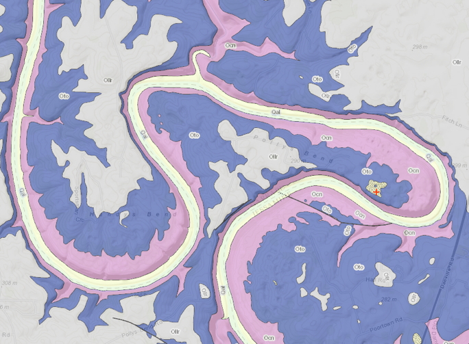
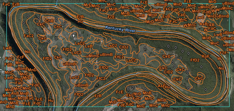
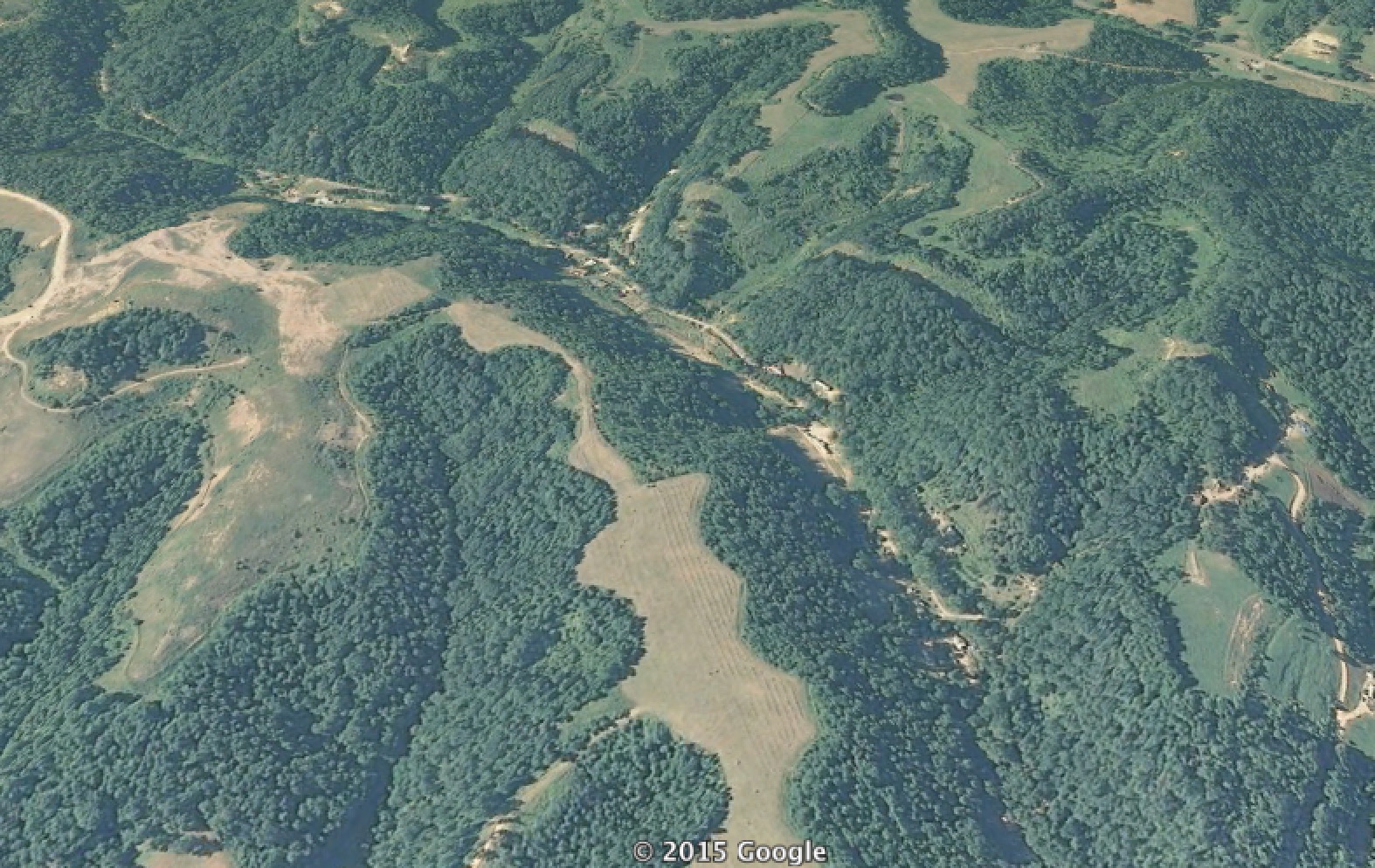
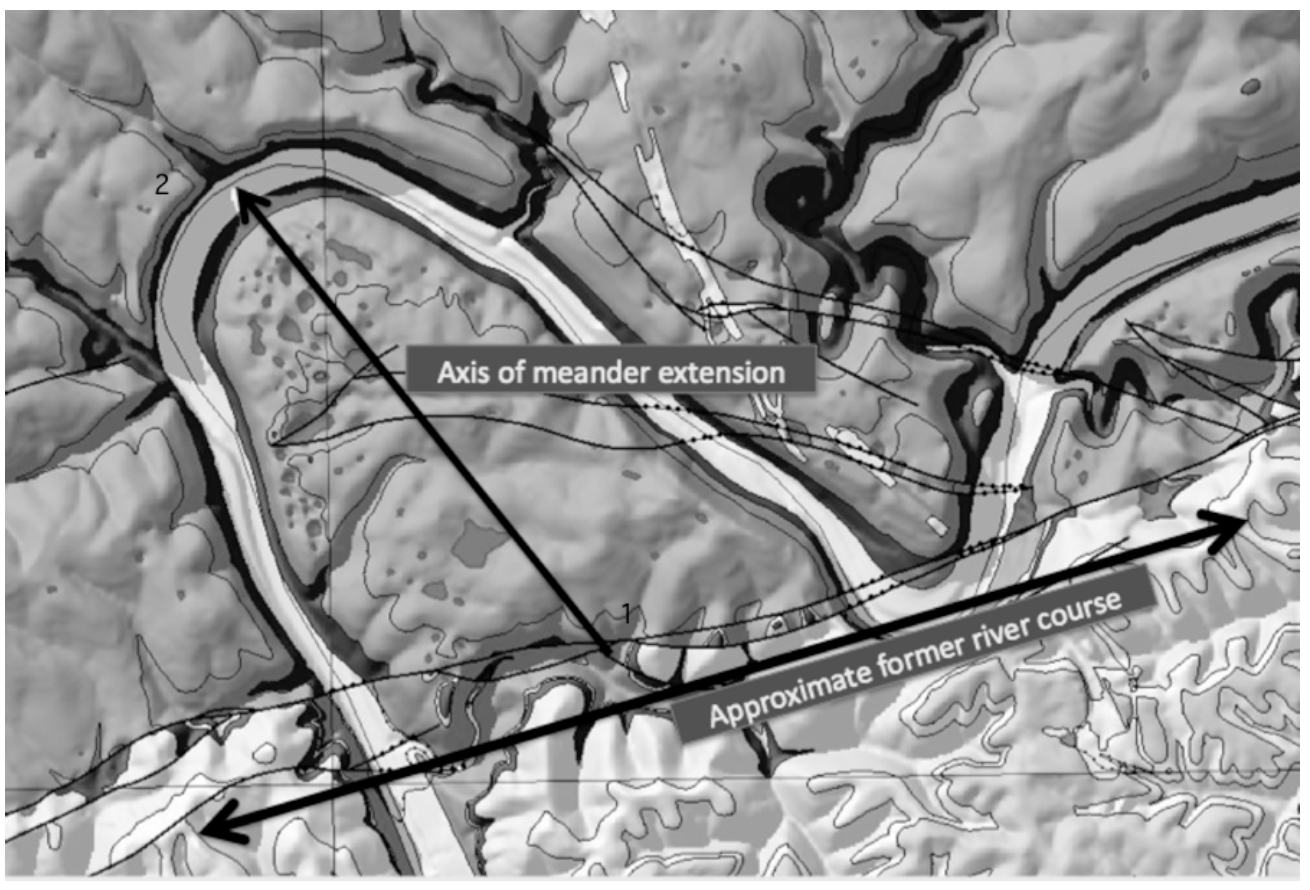
Kentucky River meander bend near Winchester, KY, chosen because high- level Quaternary terrace deposits here allow the approximate local pre-incision course to be identified. As the meander extends as shown, the direction of runoff from location 1 to the river is reversed, and the distance increases. At location 2, the distance to the river is decreased and the local slope steepened. 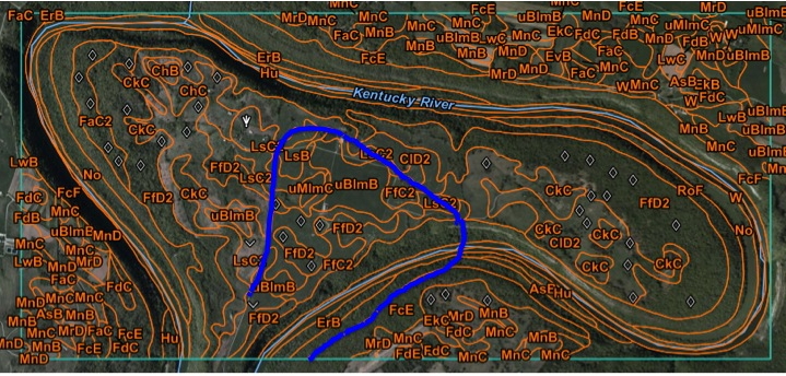Background tones on the image indicate the karst potential of the mapped geological formations, with darker colors indicating greater potential (Figure 2 from this report).

An alluvial meander grows or extends due to erosion on the outside of the bend (cutbank) coupled with accretion on the inside (point bar). In an entrenched bedrock meander, there is erosion (much of it due to slope processes) on the outer bend, though far more slowly than the bank erosion in alluvial channels. On the inside of the bend, there is a so-called slip-off slope, as the ground is beveled off by the lateral movement of the channel. You can see the slip-off slope on the inside of two of the Polly’s Bend loops in the figure below.

Topographic cross-sections across the apex of two of the Polly’s Bend meanders.

Polly’s Bend seems to have been growing during the incision of the Kentucky River gorge. In the next installment I’ll take a look at additional evidence of the growth of the bend, and exactly how much it seems to have grown.

This continues my previous post, toying with the notion of what a Romantic geomorphology would be like. This is based on the Romantic movement in art, literature, and science, rather than the more common meanings related to amourness and love, or to unrealistic idealism. Though, come to think of it, maybe Romantic geomorphology in those terms is also worth thinking about . . . .

Anyway, in the earlier post I noted that Daniel Gade’s book, Curiosity, Inquiry, and the Geographical Imagination (Peter Lang publishers, 2011) proposed 14 tenets of the Romantic imagination as it relates to research. Eight of them, in my view, apply readily to geomorphology and geosciences in general, though certainly not all practitioners display or even aspire to all of these traits.  Six others need a bit more dissection.

Search for the Exotic

Romantic scholars are drawn to anomalies and dissimilitudes. “Extreme, bizzare or grotesque patterns of the world held an uncanny attraction for the Romantic mind,” Gade writes. We can assume he refers to something beyond the interest in oddities and extremes that pretty much all humans share. He writes of research that purposefully seeks out exotic locations and situations.

Certainly this describes much of geoscience. We are inordinately drawn to the spectacular, active landscapes of, e.g., New Zealand or the Himalayas. We spend a lot of time trying to explain mysteries such as the sliding rocks of Death Valley, the fairy circles of Namibia, Uluru, and the like. We are drawn to spewing geysers, the deepest caves, the highest cliffs. What curious scientist could not wonder, and seek to learn about such things?

Fairy circles in the Namibian desert (www.express.co.uk).

However, we also have a mandate to deal with our planet as a whole, as it presents itself to us. We cannot do that by restricting our research to the places that are most scenic, fun, or exotic. In fact, those that do the (literal and figurative) dirty work of research in urban landscapes, surface mined areas, and other active and important sites that do not generally appeal to the Romantic imagination deserve a great deal of credit.

Some of us (well, me, anyway) are also coming around to a somewhat different view of exotica. The perfect landscape concept I’m always on about is based on the idea that any Earth surface system, whether the Geysers of Yellowstone, the Atacama desert, wheat fields of Ukraine, or an urban brownfield, represents a specific combination of environmental controls and a specific chain of historical events. The probability of these specific combinations occurring in any given time and place are vanishingly small. Thus to some extent they are all perfect, unique, and idiosyncratic, whether or not they are exotic.

A perfect Ukrainian wheat landscape (www. express.be).

Focus on the Particular

Romantic affinities lean toward the “particularity of the material” and prefer empiricism to theory and the local to the global. In this sense many geoscientists share the Romantic sensibility, and many do not. However, in recent years it is increasingly recognized, even among those who lean toward theory and generality, that Earth systems have irreducible elements of geographical and historical contingency (i.e., perfection in the sense above). The more Romantic geomorphologists delight in this; others may only grudgingly acknowledge it.

Characterization of Place

Much of Gade’s discussion on this point is a tirade against the straw man of positivism. Positivist was a label attached to quantitative geographers and geoscientists during the “quantitative revolution” in the mid-20^th century. It’s one of those things like “neoliberal” or “secular humanist” that are used by critics to “other” those they criticize. Very few self-identify as positivists, though many accepted the label, as it was often bandied about as characterizing anyone who is interested in measurement and not averse to mathematical and statistical methods. Few geomorphologists or quantitative geographers care much about –isms, so there was never much pushback on this label. However, if you read the literature on the scientific nature of physical geography and Earth sciences, you realize that even among the quantifiers you could classify at least as many as critical realists, pragmatists, or phenomenologists as positivists.

Anyway, though, an interest in place fits neatly with the (renewed) attention to historical and geographical contingency in geomorphology, and the Romantic geomorphologist would be right at home with it (pun intended).

Depreciation of the Obvious

Here the Romantic inquisitor is not happy with pedestrian conclusions or well-worn topics. Unexpected findings are what excite her. Again, we can assume that this means something more than the excitement over new findings and groundbreaking results that characterize any good scholar, Romantic or otherwise. The Romantic as idealized by Gade is not just pleased to happen upon such things, but is constantly pushing for them. In particular, this involves deliberately countermanding prevailing viewpoints and conventional wisdoms. Some very interesting geomorphology has been based exactly on this approach. Some of it is highly esoteric, but some very practical—for example the notion that in some environments soil erosion on steep slopes should actually be encouraged, to develop arable valley-bottom soils.

Quest for authenticity

The examples here apply to cultural landscapes and are not readily applicable to geomorphology unless you resort to some notion of naturalness unaffected by human agency, which is difficult to justify here in the Anthropocene. The Romantic prefers the real to the fake; the idiosyncratic to the standardized; the local café to the fast food chain. In terms of personal preference (as opposed to research practice), most geomorphologists are pretty earthy folks (again, pun intended), and would agree with this perspective.

Diversity for its own sake

In this section Gade focuses on cultural diversity, and the Romantic appreciation for the value and uniqueness of each and every culture. In geomorphology a perfect landscape perspective, along with the burgeoning interests in geodiversity, pedodiversity, and biodiversity, is right in line with this.

The Romantic Geomorphologist

Taking into account all 14 tenets of the Romantic scholar’s imagination, and recognizing that few individuals, be they geomorphologists, cultural-historical geographers, or anything else, are likely to exemplify all of them, I think it can be said that there exists a strong tradition and a strong contemporary strand of Romantic geomorphology. For what it's worth.

In Johnson County, Kentucky, today, lots of people along Patterson Creek are wondering “why me?”  A flash flood Monday (July 13) tore through that eastern Kentucky community, leaving three people dead, a dozen missing at one point, and destroying about 150 homes and who knows how many cars, barns, etc. (news story).

As a Kentuckian, and as a veteran of a couple of hurricanes back in 1996 in North Carolina, I sympathize with wondering why you, or your community, got hit while others didn’t. As a geomorphologist and hydrologist who was worked on flash flooding in the southern Appalachians, I also wonder about the scientific aspects—why the severe flood event in this particular location?

Make no mistake—the area around Flat Gap is not the only one in Kentucky that has gotten a lot of rain recently, and high water, runoff, soil erosion, and filled-up sinkholes are common lately throughout eastern and central Kentucky. But why the much more severe flooding at Patterson Creek?

Did they get more rain?

The eastern Kentucky climate division that includes Johnson County was recorded as having received 2.28 inches of rain July 13-15, and 3.21 in over the July 9-15 period (1 inch = 25.4 mm, the preferred SI unit for precipitation). This is about 2 inches over what would be considered normal for the period. The University of Kentucky Agricultural Weather Center’s (http://wwwagwx.ca.uky.edu) modeled precipitation maps based on observed rainfall shows the entire eastern Kentucky region with 3 to more than 4 times normal precipitation for the week ending at 19:00 (EDT) July 15. But note that some areas (Louisville vicinity, southern Ohio) are even higher:

National weather service radar-based precipitation for 08:00 am July 12 to 08:00 July 15 shows a splotch of red, indicating precipitation of 6 inches or more, exactly where the Patterson Creek flooding occurred. The 7-day radar precipitation map also shows a big red streak that includes the NW corner of Johnson County. But also note that precipitation was equally high in a number of other sites in eastern and central Kentucky that experienced no more than nuisance flooding. It is also worth noting that creeks immediately adjacent to Patterson Creek did not experience catastrophic flash flooding.

Topography and soils?

In eastern Kentucky and the southern Appalachians flash flooding is relatively common. The regional climate is such that intense frontal or thunderstorm precipitation occurs now and then. Slopes are steep and soils are generally thin, both of which tend to increase runoff and the rapidity of runoff response. Thus the region is prone to occasional flash floods, which of course can be exacerbated when surface mining, logging, and other land uses which tend to increase runoff occur.

But the Patterson Creek watershed does not appear to be atypical of the region with respect to topography or soils.

Land use

In the Google Earth image below, Patterson Creek valley is in the middle. The unforested areas you see on the ridgetops are former surface mine sites. The effects of surface mining on runoff and flooding in eastern Kentucky depend quite a bit on local details of soil, topography, vegetation, mining and reclamation practices, and local hydrology. However, the most common impact is an increase in the amount and timing of runoff, which contributes directly to flash flooding.

Patterson Creek is, alas, hardly unique within the region with respect to having been strip-mined for coal. So while the mined lands are a reasonable suspect in the recent flood, their presence alone does not explain why Patterson Creek flooded while others did not. Patterson Creek is also not unique in having residents along the valley bottom and thus vulnerable to flooding. Due to the steep slopes of the region, valley-bottom settlement is common in the region, and often the only practical option for farming or homesteading.

A perfect storm?

Likely the explanation is a combination of heavy localized precipitation (the spatial variation of which often occurs on scales too fine to show up in radar measurements) falling on already-soaked ground in an area predisposed to flash flooding, flowing into a creek which was probably running high to start with. Only detailed onsite work could even hope to settle the extent to which meteorological, topographic, soil, and land use factors contributed. Due to a relatively sparse network of rain gages, the coarse resolution of radar-based precipitation estimates, and no stream gages on Patterson Creek or any other smaller stream in the region, thus would be difficult to solve.

However, incidents such as this illustrate a broader point of the combined, interacting effect of environmental factors and history (from precipitation the previous few days to the legacy of land use) at a particular place and time to produce unexpected results. For risk and hazard management, perhaps this suggests the need to try to identify and map combinations of risk factors (such as active or reclaimed surface mines in low-order watersheds). 

The online version of my new article exploring biogeomorphology from the perspective of niche construction and extended phenotypes is now out. The abstract is below. I appreciate my colleague Daehyun Kim encouraging me to stick with some of the more speculative and provocative ideas here. I was about to back off from them at one point, but he encouraged me to go for it.

Reference: Phillips, J.D. 2015. Landforms as extended compositive phenotypes. Earth Surface Processes and Landforms DOI: 10.1002/esp.3764.