Alluvial rivers are dynamic, and often characterized by lateral migration, formation and eventual abandonment of meander loops, formation of anabranches or distributaries, and relatively abrupt shifts in channel courses. An understanding of river behavior, and effective management of resources in alluvial valleys, requires some understanding of the conditions under which these phenomena occur, and of the relationship between local and broader, reach-scale changes. This can be approached via the concept of dynamical stability.

Stability is often used in geomorphology, hydrology, and engineering in a very general sense to refer to propensity for change and resistance to perturbation. For example, a channel that shows few signs of lateral migration may be considered stable, whereas an actively laterally migrating channel may be characterized as unstable. Dynamical stability has a more rigorous and specific definition. The stability of a dynamical system (such as a river) refers to whether small perturbations tend to be diminished and damped over time, returning the system approximately to its pre-disturbance state. In dynamically unstable systems, effects of small perturbations tend to persist, and to grow disproportionately to the original magnitude of the disturbance. For instance, suppose the disturbance is a levee breach (crevasse) resulting in incision of a new channel across the floodplain. If the new channel relatively quickly infills, restoring the original channel as a single dominant channel, this represents a dynamically stable response, restoring the system to its pre-crevasse state. However, if the new channel persists as an avulsion, forming a new channel course or permanent anabranch, dynamical instability is indicated.

Lower Cape Fear River, N.C. showing multiple channels resulting from avulsions in which both channels persist (Google Earth^TM image).

Lower Brazos River near College Station, Texas showing abandoned channels near the modern river resulting from a relocation avulsion (Google Earth^TM image).

A tendency exists to categorize geomorphic systems or landforms as a whole as (un)stable. However, dynamical stability is an emergent property, in the sense that stability and instability vary with spatial and temporal scale or with the particular aspect of the system considered. For example, localized instabilities in flow-bed interactions may result in the initiation of bedforms, with resulting broader-scale stability and regularity with respect to bedform size, shape, and spacing. Consider, for example, the difference between the stability of a river reach with respect to flow bifurcations (will the bifurcation persist, or will the new channel degrade or infill?) and the stability of a flow bifurcation itself. The latter concerns whether the split flow configuration is stable, allowing both channels to persist, or unstable, whereby one of the branches will remain or become dominant while the other deteriorates. In this case, dynamical stability of a bifurcated flow is associated with dynamical instability of the reach with respect to avulsions.

An infilling channel along the Sabine River, Louisiana.

With respect to the crevasse case, Slingerland and Smith (1998; 2004) examined the stability of flow bifurcations in the sense of whether a given flow split can persist. Dynamical stability at the scale of flow hydraulics at the bifurcation results in maintenance of the flow split, and thus instability at the broader scale of reach morphology. On the other hand, instability of the flow bifurcation (leading to eventual abandonment of one of the channels) may be related to either dynamical stability or instability at the broader scale, depending on whether the original or the new channel is abandoned. The figure below shows possible local dynamically stable and unstable pathways following a levee breech.

Dynamical stability of flow splits and river channel morphology associated with levee breaches and flow bifurcations. Stable links indicate a return back toward the pre-disturbance state, while unstable paths reflect persistent changes. Contingent indicates that stability is contingent on what happens at subsequent stages.

Many scientists have noted that dynamical (in)stability at different scales may be interconnected—that is, stability at one scale may depend on instability in others. There are, no doubt, many other examples in geomorphology and hydrology.

References

Slingerland, R., Smith, N.D., 1998. Necessary conditions for a meandering-river avulsion. Geology 26, 435–438.


Slingerland, R., Smith, N.D., 2004. River avulsions and their deposits. Annual Review of Earth and Planetary Sciences 32, 257–285.


Questions, comments? Contact jdp@uky.edu

I’ve been spending a lot of time lately kayaking through tupelo/cypress (Nyssa aquatica and Taxodium distichum) swamps in eastern North Carolina, partly in connection with my continued dabbling in research, but largely for fun. I’ve also become interested in what I call “ravine swamps,” which exist along the valley side slopes of the Neuse River estuary and are dominated by tupelo gum (aka water tupelo, swamp tupelo) and bald cypress. Heck, I even own a little bit of one next to my house. 

Ravine swamp, Craven County, N.C., in winter. The scar on the foreground tree is from a floating log repeatedly bashing against it during a flood event (probably Hurricane Florence).

In my efforts to learn more about these bottomland hardwood swamps I read Status and Trends of Bottomland Hardwood Forests in the Mid-Atlantic Region (Rose and Meadows, 2016), and came across this: 

Cypress / tupelo stands are of particular concern because as these large-diameter sized stands begin to die and break up over time, they may or may not regenerate to cypress / tupelo. Both species are intolerant of shade, especially as seedlings, and require some form of fairly large-scale stand disturbance in order to regenerate successfully. In addition, developing seedlings of both species need at least a few years of dry conditions to grow tall enough to survive future flooding during the growing season. Large-diameter stands that die and break up in the absence of stand disturbance and/or during wet periods often regenerate to privet and buttonbush, resulting in a decline in the acreage of the cypress / tupelo forest type . . . .

At the same time, I’ve been wondering about the ravine swamps, the core of which have standing water year-round, which would make it difficult, if not impossible, for the key trees to regenerate. The valleys in which they formed were eroded during lower stands of sea level, and they now sit only about a meter or so above sea level and the Neuse River estuary. They could have become established when water tables were lower or during a severe, prolonged drought. But they are old enough to have had multiple generations of forest, which raises the question of how they have been maintained. 

The passage above mentions large-scale disturbance, and cypress (which has been studied more than tupelo gum) has long been known to germinate mainly in particular geomorphic settings such as infilling oxbow lakes and along channel margins. Nyssa aquatica is apparently similar in its habitat preferences, seed dispersal (both are, unsurprisingly, hydrochores, with floating seeds dispersed by water). Both can withstand constant inundation once established, but cannot regenerate from seed in flooded conditions. 

I think the key is disturbance, but not necessarily large-scale disturbance. During Hurricane Florence (2018), significant portions of the ravine swamps were covered with 0.5 to 1.0 meters of sand, turning mucky clay with frequent standing water into higher, drier surfaces (the deeper interiors of the swamps apparently got enough flushing flow from Florence’s torrential rain to keep or wash the sand out; only a thin layer remained when I got there a few days after the storm). New plants, including cypress, colonized the deposits. 

Young Taxodium distichum in sandy deposits from Hurricane Florence in September 2018, photographed in May 2021.

But this does not explain how tupelo/cypress stands are maintained in the permanently inundated interiors. As I write this area is in moderate drought, and I would still get wet up to my waist (I am almost 2 m tall) walking across the nearest one. Further, there are none of the telltale soil indicators (e.g., redox concretions) of wetland soils that dry out occasionally. While the scale of sand deposition and encroachment from Florence was unprecedented, the general phenomenon is not, as we are in an area blessed with both tropical and extratropical cyclones (nor’easters). 

One mechanism for tree reproduction that doesn’t depend on seed germination (which does not occur underwater for tupelo or cypress) is stump sprouting—a living or dead tree is broken (typically by wind during storm disturbance events) or cut and new trunks spout from the trunk. This coppice-type growth appears commonly in Nyssa aquatica. Stump sprouting can occur in bald cypress, but is rare or absent in some stands, including those hereabouts that I’ve observed. Even where it does occur, studies suggest it is not sufficient to maintain cypress numbers. Here cypress stumps do often support growth of other tree species—an example of negative ecosystem engineering?

Coppice growth from stumps, Brice's Creek near New Bern, NC

Stump sprouting, Nyssa aquatica, Neuse River

A second mechanism is uprooting (tree throw), where soil pulled out by the roots of the toppled tree is elevated above the surface, and is thus available for trees to germinate above the waterline. While tree rootwads and uproot mounds are favorable sites for new trees in many forests, it may be less so for the thin, disk-like rootwads of swamp trees, which don’t present much horizontal surface area for seeds to land on. Still, the eventual decay of the roots and resulting deposition of the sediment can leave a small mound or hummock above water level for new trees to grow on. 

Typical uprooted swamp tree, with limited horizontal surface area on rootwad for seedlings to establish.

Unidentified (but not cypress) tree growing on bald cypress stump.

The third likely main mechanism is nurse logs. Uprooting or breaking puts a trunk on the ground, in which new trees can become established as the trunk decomposes. This also seems to be quite common for tupelo gum, and rare (in my area at least) for Taxodium. 

Cypress log downed by Hurricane Florence in ravine swamp. Note also sand deposited in the wetland by storm.

The arch-like "two-footed" form of this tupelo gum indicates its origin from a seedling on a nurse log which has since decayed.

Willow oak resprouted from a downed log. 

What do all these mechanisms have in common? Trees breaking or blowing over. This can happen in moderate winds to a dying or dead tree, but most happens during tropical or extratropical cyclones. However, even in the relatively small, highly exposed ravine swamps along the Neuse, nothing approaching a stand-replacing disturbance has ever been known to occur (I can personally vouch for the past 30 years). But a handful of trees (sometimes a pretty big handful) during big storms and a single or double every now and then may be enough to maintain the tupelo/cypress swamps if we protect them from other threats. 

In the ravine swamps nearby, cypress is most common around the shallower edges, while the interiors are nearly 100 percent tupelo. Similarly, along some riverine swamps along the lowermost Neuse River upstream of the Neuse estuary the cypress are concentrated near banks, while the interior backswamps are tupelo dominated (though in both environments a number of other trees are also found, including red maple, black gum, swamp white oak, willow oak, and sycamore). Along the outer ravine swamps and river banks (which are low and often indistinct in the area I am talking about) the soil may dry out during dry spells, allowing cypress and tupelo establishment from seeds. Sediment deposition following storms or floods is also most likely in these settings. The ravine swamp interiors and lowest portions of the floodplain backswamps generally remain inundated, and thus seem to become dominated by trees that, once they gain a foothold (or roothold, I guess), are able to reproduce via stump sprouting and nurse logs. 

Some research has suggested that in the lower reaches of coastal plain rivers, as sea-level rise continues tupelo gum is likely to increase in importance at the expense of bald cypress. My observations here are consistent with that—sea-level rise means more frequent and longer inundation, which works again both trees in terms of seed sprouting, but provides a comparative advance to tupelo gum, which is better at stump and nurse log sprouting. 

Rose, A.K., Meadows, J.S. 2016. Status and Trends of Bottomland Hardwood Forests in the Mid-Atlantic Region.U.S.D.A. Forest Service, Southern Research Station, General Technical Report SRS-217.

Landscape Evolution: Landforms, Ecosystems, and Soils has been published in the electronic version, and the hardcopy will be available soon. I have mentioned previously that I wish it was less expensive--$150 list, though you can still get it for 15% less if you preorder from the publisher: https://www.elsevier.com/books/landscape-evolution/phillips/978-0-12-821725-2

While I love money (I am an American, after all), my primary desire is for people to read it.  While I was feeling a bit guilty about the price tag (though I recognize specialized books for a small audience are often pricey), I remembered that even textbooks for introductory university courses with large markets can easily run more then $100.  So I did a quick, non-scientific survey of  textbooks and a few more specialized books in areas covered in Landscape Evolution, using Amazon.com. There are many such books under 100$ (US), but many over as well. Below is a list of those with list prices of $100 or more, published since 2015. As you can see, my book is hardly in the bargain bin, but not completely out of line with the market, either. 

I would give it away if I could (I don’t expect sales to be enough for me to make much, if any, money on it once the publisher has paid their bills and taken their profits). But the folks that produced it (Elsevier) got to get paid. 

If you are wondering why I chose that publisher:

•Elsevier contacted me to see if I was interested in writing a book on landscape evolution. Beyond the ego gratification, that cuts out several steps in the dance with publishers to get a book published.

•I did not want to be constrained to produce a classroom text, or a mass-market product. Elsevier agree to that, and as a longstanding publisher of hardcore science in many fields, they know how to produce and market such works.

•I’ve had mostly good experiences with Elsevier journals, including Geomorphology, Geoderma, Catena, Ecological Modeling, Journal of Hydrology, Marine Geology, Sedimentary Geology, and Applied Geography. 

•Elsevier has been quite supportive of the Binghamton Geomorphology Symposium, a long-running (>50 years) series that I have been involved with in various ways for >30 years. 

I've attached a file that includes the book's cover (with art by Petr Mores), table of contents, and preface.

The state of an Earth surface system (ESS) is determined by three sets of factors: laws, place, and history. Laws (L=L₁, L₂, . . . , L_n) are the n general principles applicable to any such system at any time. Place factors (P=P₁, P₂, . . . , P_m) are the m relevant characteristics of the local or regional environment. History factors (H = H₁, H₂, . . . , H_q) include the previous evolutionary pathway of the ESS, its stage of development, past disturbance, and initial conditions. Geoscience investigation may focus on laws, place, or history, but ultimately all three are necessary to understand and explain ESS. 

I first started using the law-place-history (LPH) framework as a pedagogic device in my teaching, and as a sort of aide memoire framework in my research. Eventually I began invoking it more explicitly in my research and writing, and expressing it formally, as in the passage above lifted from Phillips, 2018. 

In this note I apply the framework to the overused word but vitally important concept of resilience. Resilience is the ability or potential for an ESS (or a human system) to recover from a change or disturbance. In systems theory and mathematical terms, resilience is closely, and in some contexts directly, linked to dynamical stability. In that context resilience (as recovery or tendency to return toward the pre-disturbance state) is distinct from resistance, the ability to withstand or absorb changes in inputs or external forcings. Resistance and resilience are often conflated, however, and both concepts are certainly relevant in any assessments of risk and vulnerability.

Sandy beaches are resilient to most wave and wind events, and to construction projects of my grandson Andy Phillips.

The laws influencing resilience depend on the system in question and the change or perturbation under consideration. Resilience of an agricultural system to climate warming will be governed by a different set of laws, for instance, than resilience of a barrier island to a hurricane. In general, however, the aspects of laws that most affect resilience are threefold: reversibility, system structure, and process rates. Laws determine that some processes and changes are irreversible, or not. Damage or destruction to vegetation, for instance, is in many cases reversible; vegetation can recover. Others are irreversible—the deposits from a rockfall or mudflow are not going to move back upslope. The system structure—think of an ESS as a network, and the structure as how the network is wired or connected—is closely related to, and sometimes determines, dynamical stability. The rates of processes (e.g., plant growth, soil formation, evapotranspiration) determine how rapidly a system can respond.

Specific place factors, by definition, vary greatly. Again, however, certain types of place factors are especially relevant to resilience. One has to do with the “climatology” of risks or disturbances. In some cases, climatology per se is appropriate, with respect to resilience to floods, tornadoes, tropical cyclones, and such. More generally, climatology is used here to encompass factors such as the geographically specific frequency, durations, severity, and timing of the disturbance or risk factors. You may recognize these as being closely related to the factors typically considered in studies of the geography of natural hazards. The resources available for response and recovery are also critical. In human systems these are linked to material wealth, capital, and infrastructure, as well as human experience and expertise. In non-human systems or the non-human aspects of ESS, factors such as matter and energy, geographical space, and time come into play. Yet another important category of place factors has to do with the options or degrees of freedom available—how many different possibilities are available for responding to, say, a drought or an epidemic.

I’ll also lump in here a couple of place factor categories that, strictly speaking, are associated with resistance rather than resilience. Mechanical resistance or strength relative to the force of a disturbance is self-evidently important, along with absorption capacity. 

History factors affecting resilience include initial conditions at the time of an event, such as antecedent moisture or river stages when a large rainstorm strikes, or the coincidence of natural hazards with seasonal population fluctuations. The stage of development or evolution also plays a role; some ESS are more resilient at earlier or more mature stages. The proximity of the system to thresholds is another key history factor, as is the timing and sequence of disturbance events (event history).

Most studies of resilience focus on only a few, or a single, factor. Much of my own work, for instance, has concentrated on system structure and dynamical stability, though other studies have addressed the role of history factors, and mechanical resistance. Engineers, social scientists and planners often focus on place factors. However, full understanding of resilience requires that all corners of the LPH triangle be considered. 

______________________________________

Philliips, J.D., 2017. Laws, place, history and the interpretation of landforms. Earth Surface Processes & Landforms 42: 347-354 (attached).

Posted 3 May 2021

My approach to the study of the structure, function, and evolution of Earth surface systems (landscapes) is based on the premise that they are controlled and influenced by three sets of factors, summarized as laws, place, and history. Law represents laws per se, such as the conservation of mass, energy, and momentum, and also for other generalizations and representations that are independent of location and time. Place represents the environmental context in which laws operate – ‘other things’ that are rarely equal. Path-dependent, historically contingent aspects of landscapes comprise the history. These may include sensitivity to initial conditions, previous evolutionary or developmental pathways, stages of development, disturbance histories, and time available for system development or evolution. 

My work and my approach also emphasize multiple possible evolutionary pathways and outcomes, the sensitivity of many Earth surface systems to seemingly minor variations and disturbances, and the amazing variety of landscapes resulting therefrom. These are discussed in fascinating/excruciating detail in my to-be-published-any-day-now book, Landscape Evolution.

Though the book might be the last thing I ever publish on the subject, I continue to think about it. While marveling at how Albert Collins, Roy Buchanan, Merle Haggard, Waylon Jennings, Danny Gatton, Muddy Waters, Bruce Springsteen, and Pete Townsend (among many others) could get such wonderful and different sounds from the same model of the same instrument, a Fender Telecaster electric guitar, it occurred to me that musical instruments are a fitting metaphor for landscapes. 

Early-career Pete Townsend of The Who about to smash a Telecaster. Though such smashing was his trademark in the 1960s, he reportedly spared his favorite, a 1952 Telecaster.

Bear with me on this. 

The range of sounds that can be emitted or coaxed from any given musical instrument, be it an alto saxophone, grand piano, Hammond B-3 organ or whatever, is finite and limited by fundamentals of physics and acoustics. This is directly analogous to the laws governing landscape evolution. 

These possible sounds are constrained by specific properties of the individual instrument. A Stradivarius violin presents different possibilities than the Duiffoprugcar played by legendary fiddler Vassar Clements (yeah, I just looked that up; I don’t really know much about violins) or the cheap elementary school orchestra model. The B-3 famously has a sound different even from other Hammond organs, and so on. There are also, of course, individual modifications. Electric guitarists use a variety of custom pickups (whatever those are), and of course they can be tuned differently. Bo Diddley built his style around an open-E, which has come to be called the Bo Diddley tuning. These features of individual instruments are comparable to the place factors in Earth surface systems. 

Vassar Clements and his fiddle, believed to date from the 15^th century. It was given to him by John Hartford. 

Though there are a finite (even if very large) number of sounds that can be obtained from a given instrument, there are an infinite number of potential sequences of notes or other sounds. This is the history factor. 

How many different songs are there? How many different songs could there be? And keep in mind that the same song is not always the same song. Each season of the TV show The Wire, for instance, had a different version of the Tom Waits composition Down in the Hole as the theme music. 

Comparably, we could ask how many different landscapes or landscape evolutionary trajectories exist, have existed, or could exist. The possibilities are endless. 

Of course, not every landscape song is a John Coltrane or an Allman Brothers improvisation, or even a new tune. Music can be formulaic, with certain patterns recurring because of their popularity, inherent attraction for the human ear, or suitability for a particular purpose. Baa-Baa Black Sheep; Twinkle, Twinkle, Little Star; and the Alphabet Song all have the same tune (based on a French children’s song) because it is pleasing to the young ear and easy for small children to sing. Many country trucking songs have a similar syncopated rhythm because it gives a feel of the highway. Likewise, in landscapes patterns and structures recur mainly because they are selected for in some way (efficiency selection is another major theme in my forthcoming book). 

Rahsaan Roland Kirk (1935-1977), an astounding improvisational jazz musician who could play several instruments simultaneously, at a virtuoso level. I leave the reader to ponder the landscape evolution analog of this. 

Anyway, if you want to think of landscape evolution the way that I do (and to be sure, a lot of scientists do not want to), the metaphor of landscape songs is not a bad way to start. 

-------------------------------------------------------------------

Posted 28 April 2021

Preferential flow occurs at all scales and in all phenomena in hydrological systems. By this we mean that rather than more-or-less uniform sheets of runoff moving across the ground surface, or more-or-less uniform bodies of water soaking into and seeping through soils and groundwater aquifers, most flow is concentrated in preferential flow paths.

Preferential flow of surface water—the universal tendency for flow to become channelized and form channel networks—is so obvious that it has been more or less taken for granted, though the mechanisms, and resulting structures and fluxes remain a highly active area of research. In soil and regolith, preferential flow has long been recognized, but its ubiquitous importance has only been widely recognized in recent decades. There are two main reasons for this, I think. Some forms of preferential flow, in soil pipes, large root channels, conduits, etc. are obvious, but other forms, such as macropore flow, are not readily recognized in the field. Second, a Darcian approximation of flow through porous media as a uniform mass often works fairly well, even where this type of flow is not necessarily dominant—presumably because the local preferential flow variations tend to average out in the aggregate.

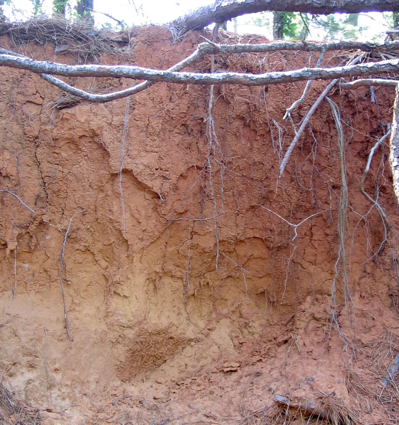
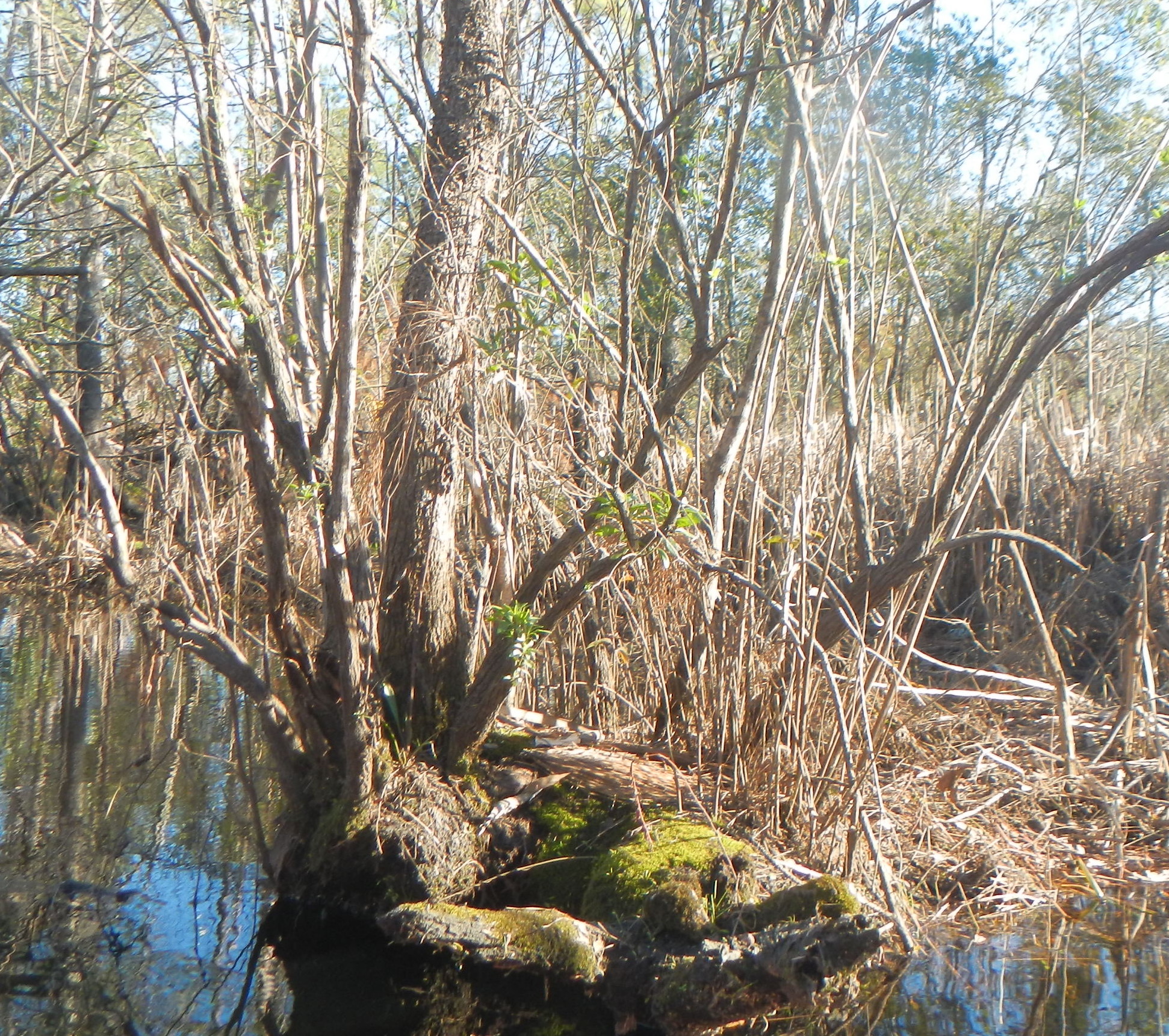
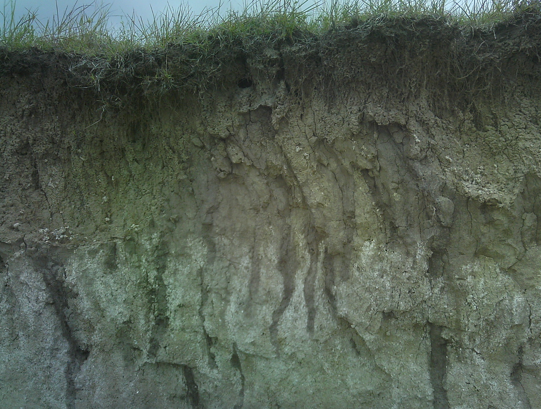
An Ultisol in southwestern Louisiana. Like many soils, preferential flow paths are not necessarily evident at a cursory glance. Look more closely, however, and you seem numerous structural cracks, pin-hole to pencil-size pores, and roots & root channels.

But preferential soil moisture flux is ubiquitous, and may even occur (due to unstable wetting fronts) in relatively uniform sands. Preferential flow also occurs in various kinds of macropores and cracks, associated with, e.g., insect burrows, fine roots and root traces, interconnected soil pores, boundaries of soil aggregates and rock fragments, etc. For convenience I will use macropore to encompass all of these.

Sandy soil in coastal south Texas showing morphological evidence of preferential “fingered flow.”

In the last decade or so, substantial evidence has emerged that many soils (and groundwater systems) develop a dual-porosity structure, with slow flow and sometimes extensive storage in the matrix, and rapid flow with limited or transitory storage in macropores.

Henry Lin (2010) linked subsurface flow regimes and pedogenesis, pointing out that the dual partitioning of matrix and preferential paths goes a long way toward explaining the genesis of soil structure. He interpreted this in terms of the interplay of dissipating and organizing processes, and pointed out that the constructal theory of flux paths also predicts evolution toward flow partitioning and dual porosity.

Worthington (2019), working with groundwater systems, found that a high resistance matrix and low resistance preferential flow paths together form the minimum overall flow resistance; greater than that of a single-porosity system. There is in essence a division of hydrological labor, with the matrix taking care of storage and the preferential flow paths doing most of the transport work. The same phenomenon has also been interpreted in terms of coevolution of ecosystems, soils, and hydrology to satisfy contrasting hydrological functions of efficient drainage and sufficient storage of water and nutrients (Savenjie and Hrachowitz, 2017).

All of this makes perfect intuitive sense to me, is consistent with my field observations, and is supported by a great deal of empirical, model, and theoretical evidence. But I still have a bit of trouble wrapping my head around how it works at scales or conceptual levels in between the overarching principles of efficiency selection and organizing and dissipating processes, and the measurable particulars of a specific site or system.

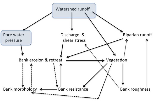
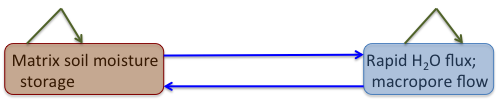
Let’s consider the relationship between slow flow and soil moisture storage in the matrix, and rapid macropore flow. In any soil or hydrologic system, there is a given amount of available water in the form of excess precipitation. As a first approximation, partitioning this between matrix and macropores is a zero-sum game, and the two components can be considered competitive, with minus signs on the blue arrows in the figure below. That is, any H₂O stored in the soil reduces the potential macropore flow, and vice-versa. The green arrows indicate self-effects; intrinsic constraints on the upper or lower values for negative self-effects, and positive feedbacks (self-reinforcement) for positive self-effects. Examples of some self-effects are shown in the table below.

With both self-effects negative, the system is dynamically unstable, indicating that a change will tip the system away from its pre-perturbation state—unless either component is near one of its limiting states, and these self-effects are stronger than the competitive relationship between the components. Suppose, for example, that soil moisture storage is approaching field capacity. Soil moisture is thus not competing with macropore flow, and increased macropore flow has little impact on soil moisture. The system tips to a saturated soil, macropore flow dominated state, allowing the excess moisture to drain away. This dynamically stable state exists until something (e.g., a change in the weather, rise of the water table to the surface) modifies the relationships (i.e., changes the sign of the green or blue arrows).

In another scenario we start with dry soil, with soil moisture at the wilting point—this negative self-effect dominates the system, as there is no macropore flow and no moisture to compete for. The beginning of a wetting event favors soil moisture, which wins the competition for water (limiting macropore flux), and may also switch to positive feedback as wetting fronts advance. This instability switches the system to a soil-wetting, limited macropore flux state. As (or if) soil moisture continues to increase, macropore flow comes into play and starts seriously competing with matrix storage, and stability is regained.

Yet another scenario is a super-wet state—the soil is saturated and maximum macropore flow is occurring, with the water table at or near the surface. Both self-effects are negative, but flow competition is irrelevant, creating a neutrally stable condition. After water input ceases, however, macropore flow begins to win the competition, with instability tipping the system to a wet soil, macropore dominated state. This facilitates more rapid drainage.

Other scenarios are possible, but these examples illustrate how the presence of both matrix storage and macropore flow allow the system to adjust to changing hydroclimatic conditions. Note that dynamical instability is necessary to allow the soil hydrological system to switch between different states.

But how, exactly, does the dual-porosity come into being?

Broadly speaking, it is a two-stage process. First, openings or macropores are created or the soil is segregated into high-resistance, tightly packed zones, and low-resistance potential flow pathways (PFP). Then preferential flow itself causes the dual porosity structure to persist (and in some cases become more pronounced).

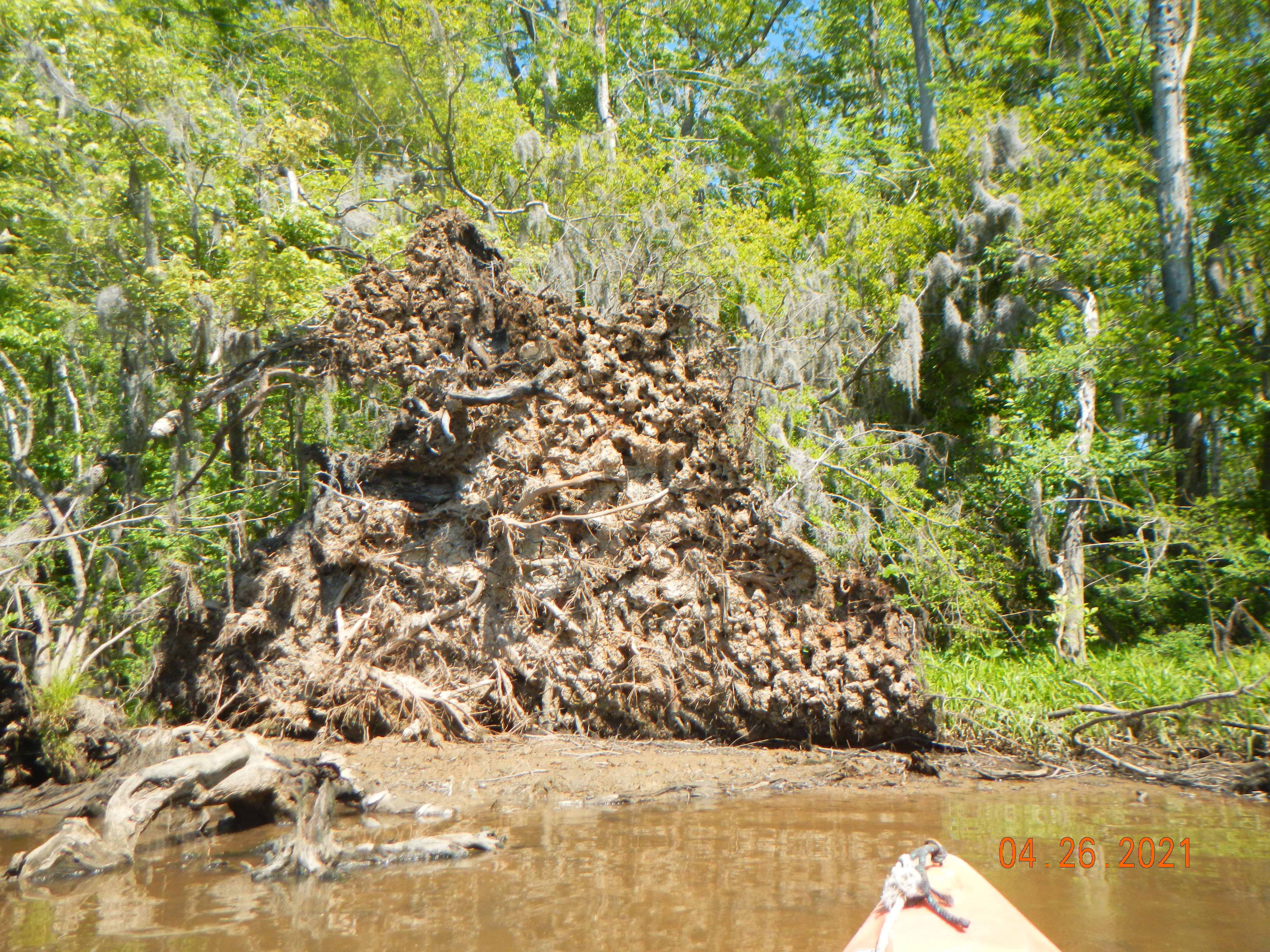
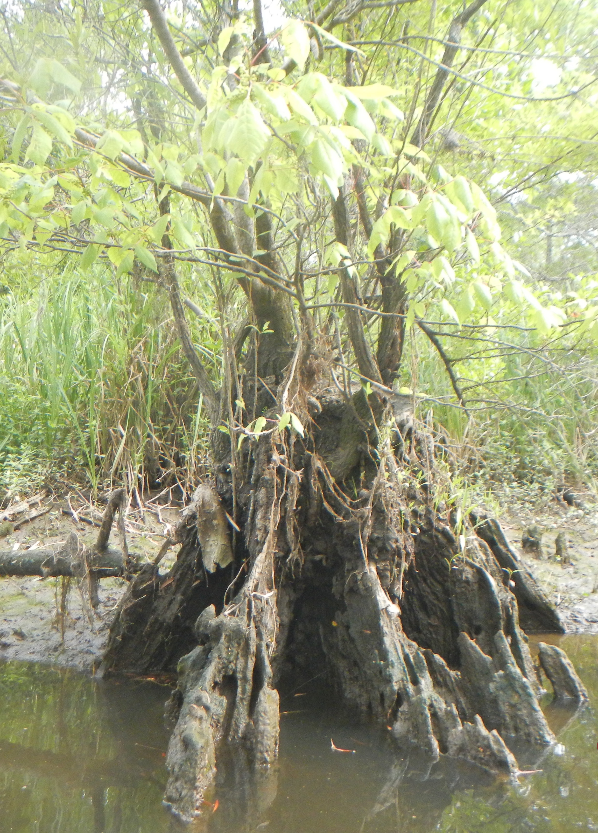
The stage one segregation can occur due to a number of physical phenomena, including grain-packing, gravitational settling, shrink-swell and freeze-thaw processes, and boundaries or partings inherited from parent material. More important in many settings are biological processes, such as faunal tunneling and burrowing. Most important and interesting of all, to me, are the effects of plant roots, both exploiting, creating, and expanding PFPs.

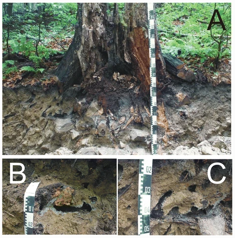
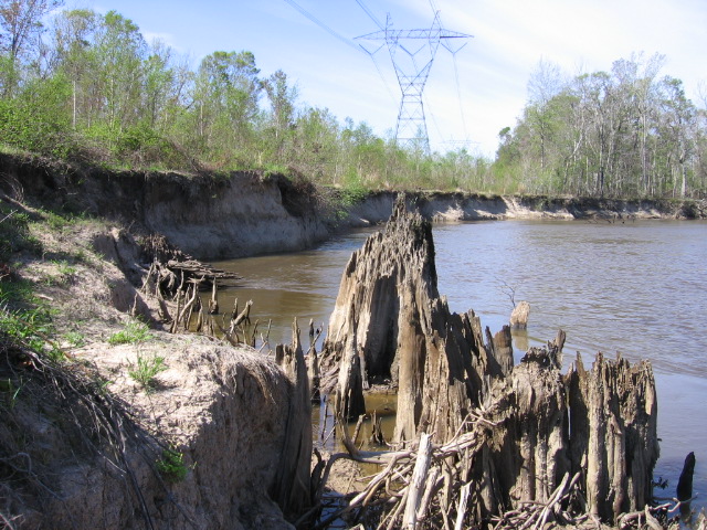
Fig. 5 from Pawlik & Šamonil (2018): beech stump in a Haplic Cambisol, Turbacz, Gorce, Poland. a – general view, b – decaying roots and empty root channels, c – dense network of root channels

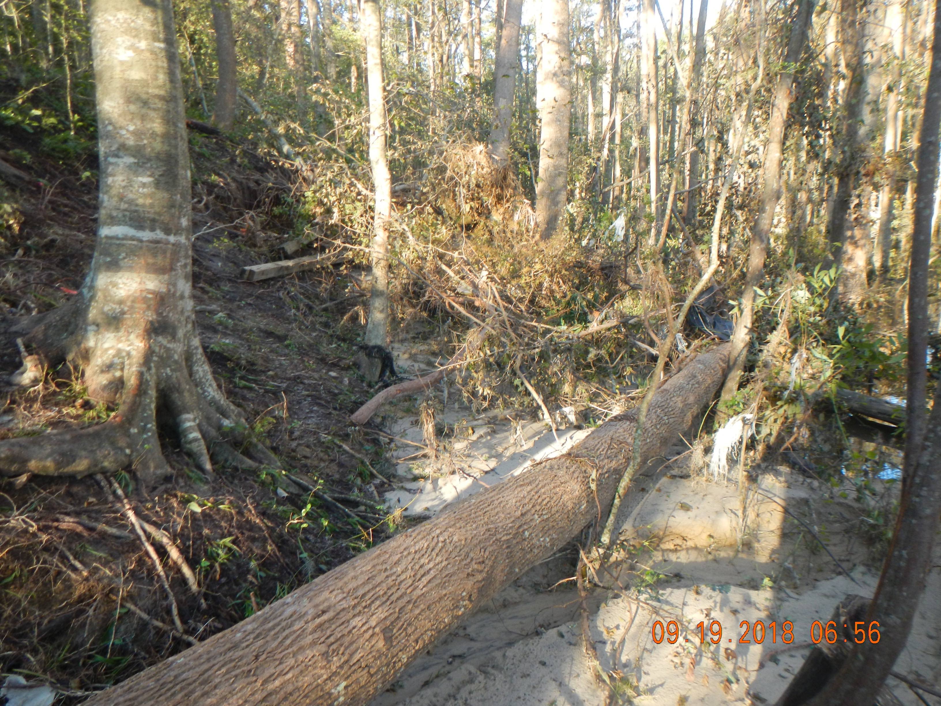
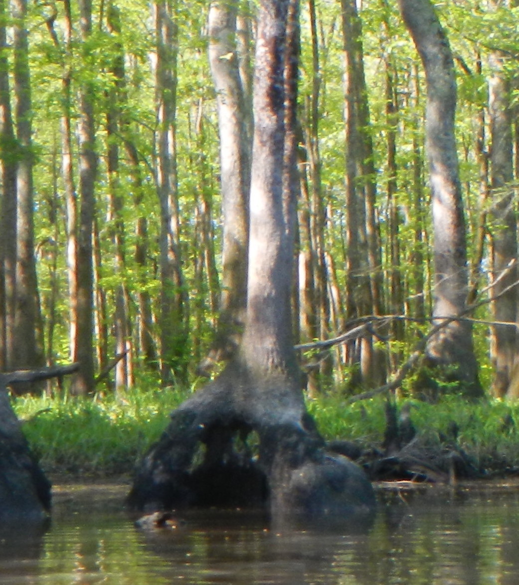
Persistence and potential growth of PFPs can occur due to mass transport and erosion (physical and chemical) along the PFPs. Certainly macropore deposition and clogging can occur, but the overall net effect is to maintain and sometimes enlarge the PFPs. With respect to biological features, fauna may maintain their tunnels. Plant roots both funnel infiltrated water along roots, and extract water via transpiration along these pathways. In addition, the roots and the associated microbes in the rhizosphere create chemical conditions that facilitate weathering and dissolved material transport. The pressure of root growth pushes soil material aside, packing it more tightly and reinforcing the high-flow-resistance matrix.

The specific details of these processes are highly variable, but one very recent and specific example examines changes in podzol morphology due to tree root modification of soil hydrology and porosity in a tropical rainforest in Brazil (Martinez et al., 2021). Pawlik and Šamonil (2018) showed how hydromorphic processes associated with tree roots persist in podzolized soils in three temperate forest settings, in ways consistent with development of dual porosity systems. Brantley et al. (2017) give an overview of how trees “build and plumb” the critical zone.

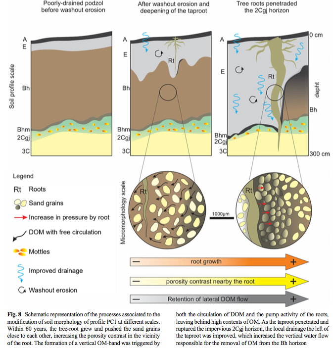
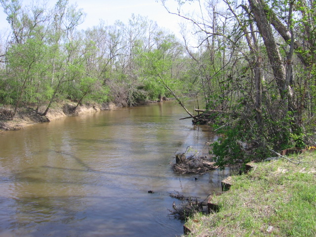
From Martinez et al., 2021

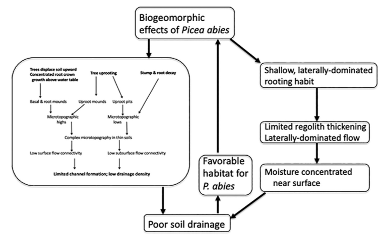
So plants, especially trees, help create dual-porosity soil and regoliths. This, in turn, provides a soil moisture storage reservoir for plants in the form of the matrix, and a mechanism for rapid drainage of excess water via the PFPs.  This is, therefore, an excellent example of positive ecosystem engineering, and the coevolution of soil, hydrologic, and ecosystems.

References

Brantley SL, Eissenstat DM, Marshall JA, et al. 2017. Reviews and syntheses: on the roles trees play in building and plumbing the critical zone. Biogeosciences 14:5115–5142

Lin, H., 2010. Linking principles of soil formation and flow regimes. Journal of Hydrology 393: 3–19.

Martinez, P., Buurman, P., do Nascimento, D.L., et al. 2021. Substantial changes in podzol morphology after tree‐roots modify soil porosity and hydrology in a tropical coastal rainforest. Plant and Soil: https://doi.org/10.1007/s11104-021-04896-y.

Pawlik, L.,  Šamonil, P., 2018. Biomechanical and biochemical effects recorded in the tree root zone – soil memory, historical contingency and soil evolution under trees. Plant and Soil 426, 109-134.

Savenjie, H.H.G., Hrachowitz, M., 2017. HESS opinions: Catchments as meta-organisms—a new blueprint for hydrological modeling. Hydrology and Earth System Sciences 21: 1107-1116.

Worthington, S.R.H. 2019. How preferential flow delivers pre-event groundwater rapidly to streams. Hydrological Processes 33: 2373-2380.

Comments/questions: jdp@uky.edu

Several years back when I was working on the energetics of landscape evolution, focusing on the biological subsidy to geophysical energy sources, I tried to get my head around the energy required to turn fresh rock into transportable debris by weathering. I looked at factors such as the chemical activation energy of rocks, and various strength/stress measures (tensile & compressive strength, etc.). My geochemistry and rock mechanics background is/was too feeble for me to get very far with this beyond drawing two very broad conclusions:

1. It takes a lot of energy to break down rock.

2. There has to be more to it than the basic force/resistance principles (for example shear stress vs. shear strength) that I am familiar with, and that work perfectly well in some contexts. 

Breaking rocks the hard way

The answer to item 2 (or at least ananswer) came in the form of the concept of subcriticalstresses and processes. I have not done a deep dive into the origins of these concepts, but arguably the pioneer (and unarguably my gateway to it) is M.-C. “Missy” Eppes. Though she had worked on the concept before, a 2017 article with Russell Keanini introduced me to weathering due to subcritical cracking. 

Their analysis of fracture mechanics established that mechanical weathering in most rock types progresses by climate-dependent subcritical cracking under virtually all Earth surface and near-surface environmental conditions. Eppes and Keanini (2017) developed subcritical cracking and rock erosion models based on fracture mechanics and mechanical weathering theory and observations. They showed that subcritical cracking can culminate in significant rock fracture and erosion under commonly experienced environmental stress magnitudes that are significantly lower than rock critical strength. 

Eppes and Keanini (2017) were particularly concerned with climate effects, and their results indicate that climate strongly influences subcritical cracking—and thus rock weathering rates—irrespective of the source of the stress (e.g., freezing, thermal cycling, and unloading). The climate dependence of subcritical cracking rates is due to physical and chemical processes acting to break bonds at crack tips experiencing these low stresses. They found that for any stress or combination of stresses lower than a rock’s critical strength, linear increases in humidity lead to exponential acceleration of subcritical cracking and rock erosion. 

Figure 1 from Eppes & Keanini (2017)

The take-home message for me was that macro-thresholds (that is, applicable to an entire rock mass or clast) of force-resistance do not have to be exceeded for weathering and erosion to occur. Micro-scale thresholds of bond-breaking in tiny cracks can also get the job done. 

In a commentary titled “breaking rocks made easy,” Voigtländer and Krautblatter (2019) related subcritical cracking and stress at the microscale within rocks to the broader scale stress fields associated with tectonics (the tectonic predesign principle pioneered by Adrian Scheidegger).  I cannot do a better job than they did in explaining (including a delightful series of cartoons) how concentrations of stress at key points can get erosional work done even when overall force:resistance thresholds (that is, those that can be measured at scales larger than the micro- or nano-scale) are not exceeded. This includes the direction at which force is applied in addition to heterogeneities in the material. 

Two of the cartoons from Voigtländer and Krautblatter (2019) using simple analogs. 

Tectonic geomorphology and rock mechanics are not my areas of expertise, but in thinking about riverbank erosion processes in my previous post, the general reasoning probably applies to weathering and erosion more general—that is, the important action may occur at very local (subcritical) scales. Erosion resistance can be controlled by, say, the loosest grain or aggregate or the invisible crack in the rock rather than by what could be measured with, for instance, a shear vane or a Schmidt hammer. 

This switches my original question from “why are (traditional) force:resistance analyses so often unsatisfactory?” to why they work as well as they do, given the unbiquitous anisotropy and heterogeneity in even the most uniform-appearing Earth materials and the presence of invisible stress fields. 

I don’t have even a proposed answer for this at the moment, but it leads me to another analogy: the local nature of efficiency selection. Many flow processes (and other processes, too) are governed by a general principle whereby more efficient flow paths tend to persist and grow, while less efficient ones do not. But flowing or seeping water, growing root tips, creeping soil, etc., can only “see” and react to what is in their immediate vicinity. Thus the most efficient local path may or may not be consistent with the most efficient configuration at the broader scale of a channel or conduit network, root system, or hillslope. Tasnuba Jerin and I presented an example of this in a fluviokarst system (Jerin and Phillips, 2017). 

Tasnuba Jerin (front) and Darion Carden contemplating local efficiency selection in a paleochannel of Shawnee Run, Kentucky.

Eppes, M-C., Keanini, R. 2017. Mechanical weathering and rock erosion by climate-dependent subcritical cracking. Reviews of Geophysics5: 470–508, doi:10.1002/2017RG000557. 


Jerin, T., Phillips, J.D., 2017. Local efficiency in fluvial systems: Lessons from Icicle Bend. Geomorphology282: 119-130. 

Voigtländer, A., Krautblatter, M. 2019. Breaking rocks made easy. Blending stress control concepts to advance geomorphology. Earth Surface Processes & Landforms44: 381-388, doi:10.1002/esp.4506.

Questions/comments: jdp@uky.edu

River and stream bank erosion is normally assessed—including studies I was involved in--by reaches. That is, the erosional (or stable or accreting) status is assessed along sample reaches of a certain length (e.g., 100 m long segments), or lengths of shoreline are classified—e.g., a 40 m erosional stretch, a 120 m stable stretch, 30 m accreting length, etc. Or, where rates are measured, they are presented (not illogically) as mean or characteristic values for a reach.  They are also generally averaged over time—so, for example, if the bank retreated 1 m in a decade, a rate of 0.1 m yr^-1 is reported. Again, in many cases that is entirely reasonable, as (depending on the study design) there is often no way of knowing for sure if the erosion occurred at a more-or-less steady rate, all in one flow event, or somewhere in between. For some alluvial streambanks, there also exists uncertainty as to whether the observed retreat represents nothing but erosion, as opposed to net erosion—for instance, 1.5 m of retreat over 10 years, offset by 0.5 m of accretion somewhere during that time.

Eroding banks, Old River, Louisiana.

A recent e-mail exchange with a fluvial geomorphologist colleague got me thinking about this. He pointed out that in his data, which overcomes the main limitations above, shows many years of zero erosion even along banks undergoing general long term erosion, and often very little relationship between erosion and the magnitude of flood events.

Geomorphic change is often episodic, with long periods of little or no change interrupted by episodes of sometimes rapid change, so that aspect is not entirely surprising (though many banks undergoing long term net erosion certainly appear to be consistently vulnerable—for example where weak bank material on a steep slope with limited vegetation cover or debris protection is exposed). Disproportionate responses to forcing events are also well known in fluvial geomorphology—that is, big floods with limited geomorphic impacts and smaller flows with disproportionately large impacts.  And complex responses and high degrees of local spatial variability are also widely recognized in fluvial geomorphology.

Indian Bayou, Texas, showing different dominant modes of bank erosion on opposite banks, and local variations in morphology and apparent retreat on both sides.

We know that in addition to the magnitude of a flood event (the discharge, stream power, etc.), the timing and sequence of events and the resisting framework are important in determining impacts—and even at a single point on a stream bank the latter may change as bank vegetation, woody debris, and morphology change. We also know that thresholds are important—for instance, if a stream bank has developed an overhang that is near its critical failure point, it may not take much to initiate a collapse.

Reach of Shawnee Run, Kentucky showing banks with evidence of erosion, accretion, stability, and erosion-recovery within a small area.

The upshot is that rates of bank erosion (or other change) and aspects of bank morphology, vegetation, etc. tend to be highly spatially complex, with a great deal of local variability over short distances. Fonstad and Marcus (2003) found that the distribution of bank failure sizes conforms to self-organized criticality (SOC). The power-law size-frequency distributions that are the signature of SOC can arise from several different causes, but Fonstad and Marcus (2003) linked their findings to complex nonlinear dynamics among the processes and controls of bank erosion. Croke et al. (2015) found the evidence for SOC in bank failures following a major flood to be equivocal, but with clear evidence of nonlinear dynamics, high spatial variability, and disproportionate responses relative to the magnitude of events. They also noted that defining a critical state is no easy tasks when multiple modes of adjustment and numerous feedbacks are present.

So, I did what I do—a combination of abstract theory and muddy-boots field evidence. The figure below represents the interactions among key factors. Watershed runoff represents the supply of water to the stream system, a function of the hydroclimatic water balance and runoff response. This considers not only runoff that appears as channel flow (discharge), but also as local runoff across stream banks (riparian runoff) and groundwater in the vicinity of banks (pore water pressure). The vegetation factor includes with living vegetation and woody debris and relict stumps and roots that affect hydraulic roughness, bank morphology, and resistance (e.g. shear strength).

Interactions among key factors in stream bank erosion. Watershed runoff and pore water pressure are highlighted because they are external factors in that they do not directly influence system stability. Thicker arrows indicate positive links (an increase or decrease in the source component leads to a change in the same direction in the other component), and thinner arrows negative links (increases or decreases have inverse effects). Dotted arrows indicate effects that may be either positive or negative with respect to bank erosion.

This kind of model can be assessed using the Routh-Hurwitz criteria to assess its dynamical stability, based on the eigenvalues of the interaction matrix. I analyzed the matrix for the system shown here, using various combinations of negative and positive for the dotted-line arrows. The bottom line is that there is no dynamically stable configuration, even under various assumptions of relative strengths of various lengths, and assuming that some components have stability-increasing self-limiting affects (not shown on the diagram for the sake of clarity).

This dynamical instability implies that following a change to any component—e.g., erosion or deposition that modifies bank morphology; addition or removal of vegetation or woody debris; changes in resistance or riparian runoff response due to creation or exposure of different materials or surfaces—the stream bank system is unlikely to return to its previous state. Dynamical stability also implies sensitivity to variations in initial conditions.

Students in my 2017 fluvial geomorphology class in Shawnee Run, Kentucky. Bank in the background is undergoing net long term erosion, but extensive local variation in bank morphology, material, roughness, resistance and vegetation is evident.

Complex, variable (in time and space) stream bank changes are inevitable, at least at the scale at which the interactions shown in the model hold. This does not preclude stability at broader scales; nor does it invalidate all-other-things-being-equal principles relating to individual relationships—for instance, other things being equal, lower bank resistance leads to more erosion.  This result also indicates the need to pay attention to local variations in the key factors and proximity to thresholds, and to expect disproportionate responses and local spatial variability.

Sabine River, Texas/Louisiana, showing formerly eroding bank now at least temporarily stabilized and featuring recent deposition.

References

Croke, J., Denham, R., Thompson, C., Grove, J. 2015. Evidence of Self‐Organized Criticality in riverbank mass failures: a matter of perspective? Earth Surface Processes & Landforms 40, 953-964.

Fonstad, M., Marcus, W.A. 2003. Self-organized criticality in riverbank systems. Annals of the Association of American Geographers 93: 281-296.

Questions/comments: jdp@uky.edu

Just published in Geomorphology, with Pavel Šamonil: Biogeomorphological domination of forest landscapes: An example from the Šumava Mountains, Czech Republic.

This paper originated from a more general study of forest biogeomorphology in unmanaged forests of the Czech Republic. In higher elevations and upper slopes mainly in the Šumava National Park, we noticed an almost complete lack of stream channels and surface runoff, except on or near roads and associated drainage features (and in the valley bottoms).

Pavel Šamonil (right) and yours truly.

In attempting to explain this, which I originally thought was a distraction from the main mission, it emerged that biogeomorphic effects of Norway spruce are responsible for the lack of surface drainage, as well as other geomorphic and hydrological phenomena. One headline, beyond a very interesting regional landscape evolution story, isthat biogeomorphological feedback domination of landform and ecosystem development can last for an extended period of time (rather than a relatively limited successional phase).  Some other potential examples of the same phenomenon are cited in the literature review in the paper (attached).

Figure 13 from the paper, summarizing how biogeomorphic effects of Picea abies maintain favorable habitats for the species.

Another headline has to do with the biogeomorphic ecosystem engineering (BEE) effects of Picea abies. BEE by trees is well established, and is often advantageous to the engineer species. However, it has been difficult to show that the beneficial BEE effects are specific to the engineer species, as opposed to trees more generally. In this case, however, the BEE effects of spruce help maintain habitats that give a clear competitive advantage to Picea over other potential vegetation competitors.

Pavla Cizková (top, center) and Pavel Hubený (bottom) provided moral and logistical support, DEM data, and face paint for the research effort.

__________________________________

Phillips, J.D., Šamonil, P. 2021. Biogeomorphological domination of forest landscapes: An example from the Šumava Mountains, Czech Republic.  Geomorphology 383: 107698 (attached).

Questions/comments: jdp@uky.edu

Elsevier has announced a May 1 predicted shipping date for my forthcoming book, Landscape Evolution, cheerfully assuming that someone will want it. Below is the mockup of the back and front covers, complete with descriptive blurb and cover art by Petr Mores. You can pre-order at https://www.elsevier.com/books/landscape-evolution/phillips/978-0-12-821725-2.

I will admit that I am not entirely comfortable with the suggested price of US $150, but that's the way it goes for specialized academic tomes with a limited market. However, the book will also be available in electronic format, and if your library gets it (although many university libraries are enduring drastic budget cuts of late), I understand you will be able to access a chapter at a time in pdf form. And you can get it cheaper if you pre-order. Once it is out, if you really want to see it and can't afford it or access it through a library, contact me and I will try to help. I would love for people to buy it, but it is much more important to me that someone reads it!

Questions/Comments: jdp@uky.edu