As I write, river flooding and cleanup from Hurricane Florence in North and  South Carolina are ongoing. The storm was not a major one in terms of maximum sustained winds--only a Category 1 on the Saffir-Simpson scale when it made landfall at Wrightsville Beach, near Cape Fear, NC.  But the storm approached the coast very slowly, and moved only very slowly once it made landfall. That, and the areal extent of of the storm, resulted in quite a beating for the eastern Carolinas. 

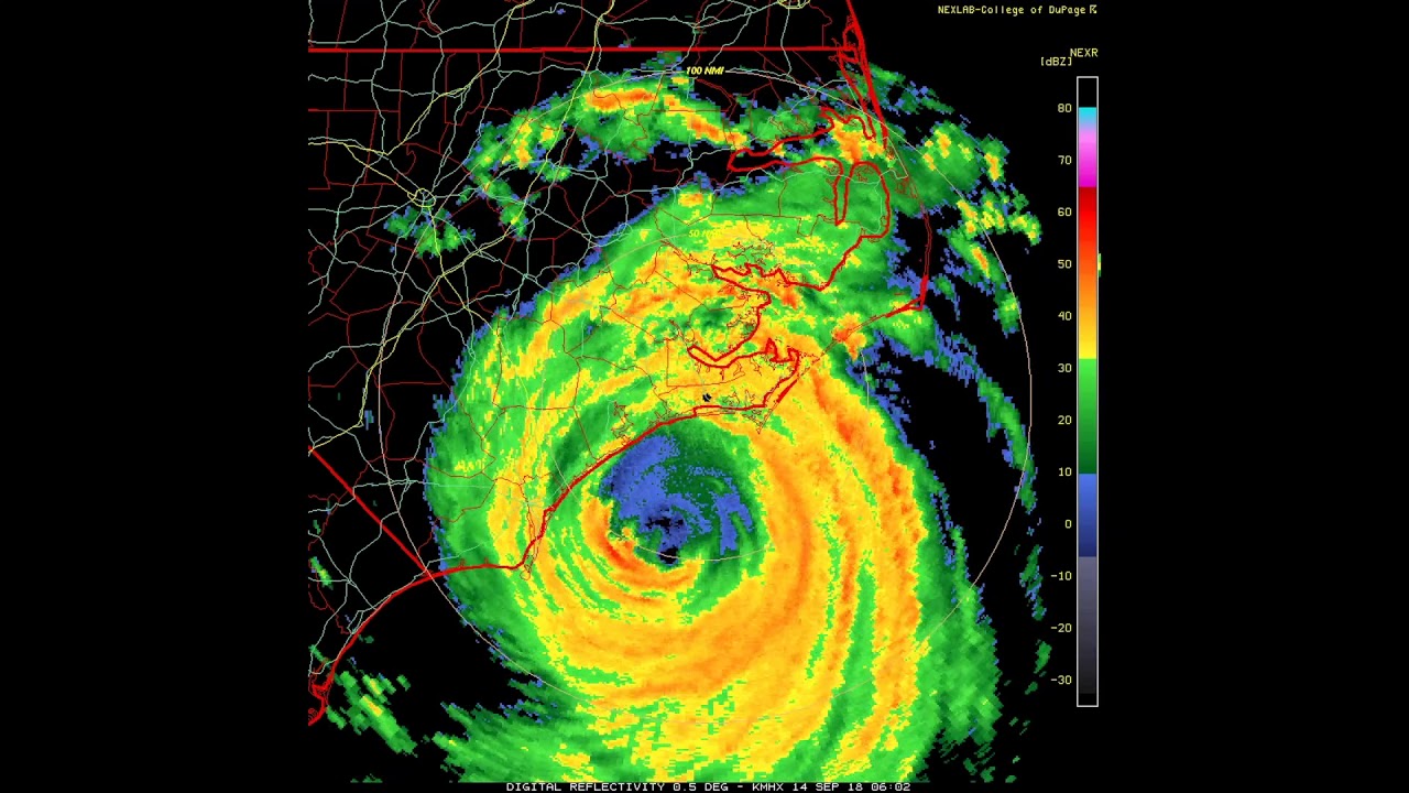
Satellite image of Florence approaching the Carolina coast. 

The slow movement allowed the tropical cyclone to continue recharging its rain bands with warm, moist air from the Atlantic Ocean, resulting in 17 to 36 inches (432-914 mm) of rain in coastal N.C., and >10 inches (>250 mm) in many inland locations, in the middle and upper portions of the river basins. With respect to river flooding in the Carolinas, Florence draws comparisons to Hurricanes Floyd (1999) and Matthew (2016). The record peaks in most rivers of the have now occurred in one of those three events. But in the cases of Floyd and Matthew, the rain was falling on ground that was already wet and running off into streams that were already running high--in other words, the antecedent conditions made the flooding far more extensive than it would have been otherwise. Florence was different. As it approached the coast, conditions were relatively dry, and streams were at lower flow ranges (as they often are in September).  Thus in terms of the hydroclimatological synoptic situation, Florence reminded me much more of Hurricane Harvey, which struck the Texas Coast in 2017. 

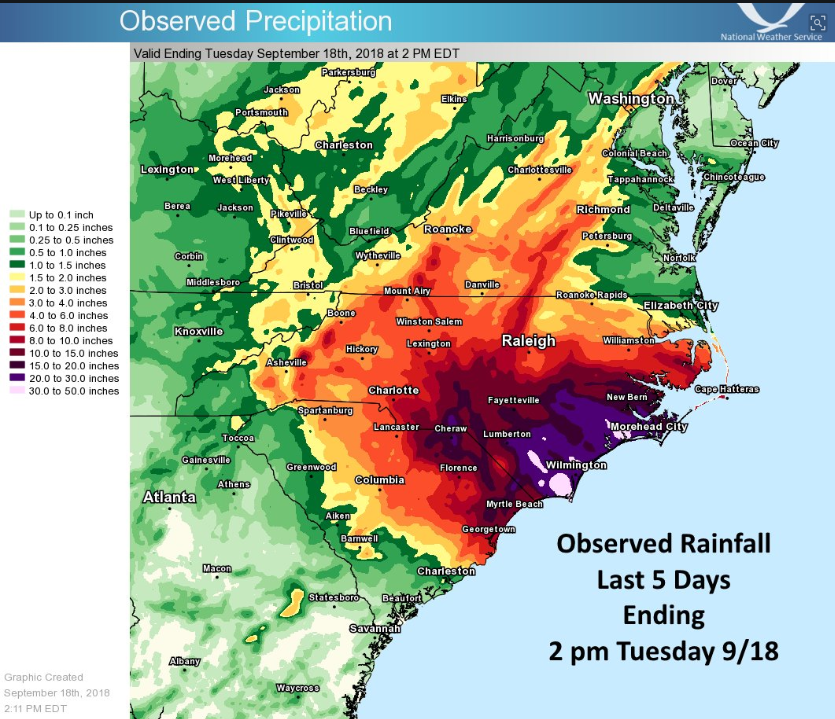
Rainfall from Florence (National Weather Service, Newport/Morehead City NC). 

Harvey resulted in record storm rainfall totals for the USA; >50 inches (>1270 mm) in numerous locations, and massive rainfall flooding (in addition to wind, wave, and storm surge effects). While Harvey was a much larger storm than Florence in most respects, they had two things in common--very slow movement, and very large areal extent.  The National Hurricane Center’s report on Harvey is here, and the U.S. Geological Survey’s study of flooding resulting from the storm is here.

A recent study showed that hurricanes have slowed their rate of movement by 10% in recent decades--and that doesn't include Harvey and Florence. The cyclone slowdown is consistent with a weakening in atmospheric circulation in the tropical parts of the planet, a result of global warming, study author James Kossin found.  However, the mechanism behind the slowdowns are unclear.

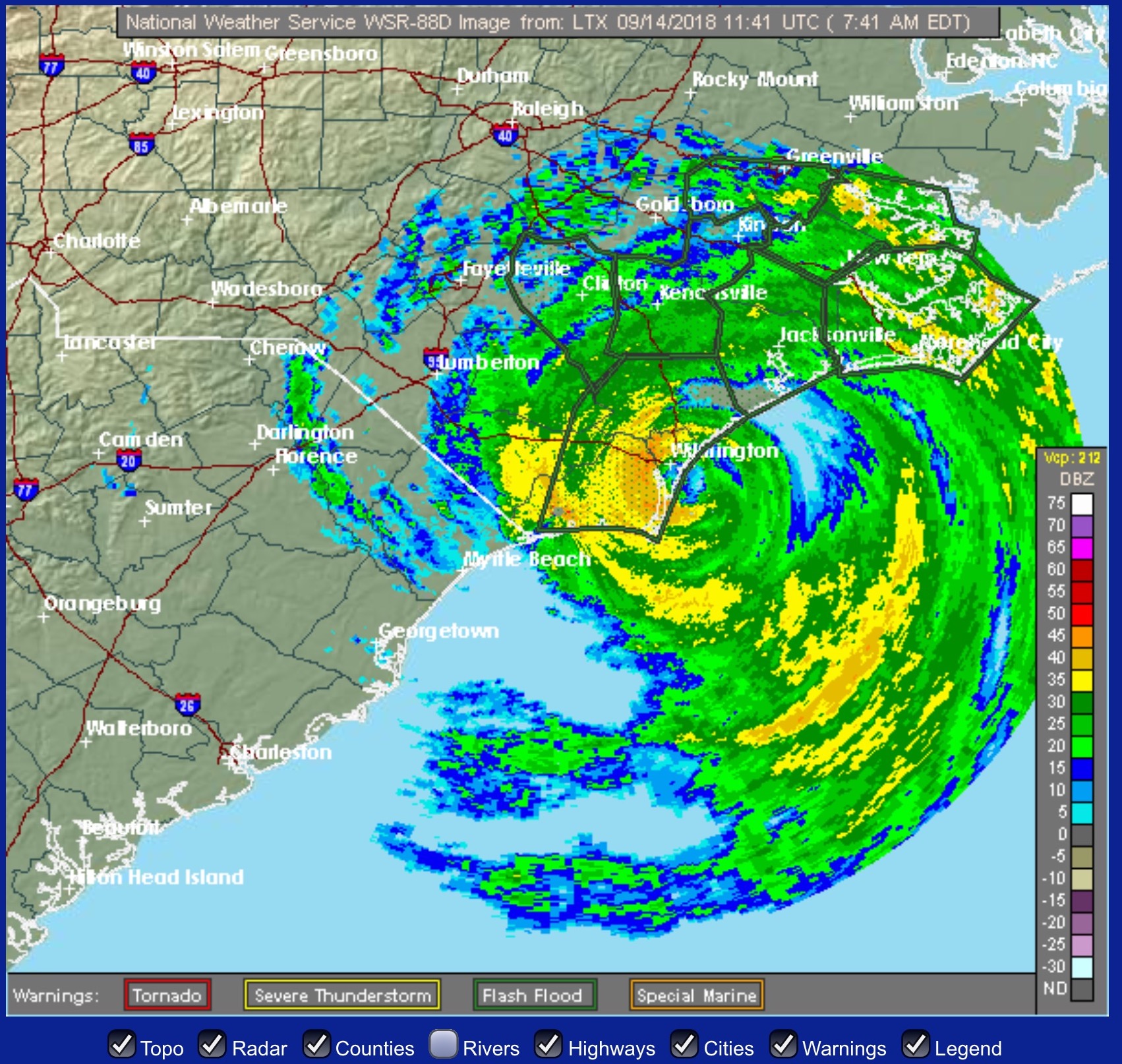
Radar image at landfall. The storm moved only very slowly (about 8 km/hr) as it approached the coast and moved inland. 

Regardless of what may be slowing down hurricanes, we can expect things to get worse (or better, if you like tropical cyclones) as the climate warms. It is well established that warm water is necessary for tropical cyclone development, and once formed, tropical storms are fueled by warmer water. Further, each 1 degree C increase in air temperature results in a 7 percent increase in saturation vapor pressure and how much water vapor the air can hold. This both provides more fuel for hurricanes (as release of latent heat as moisture condenses in the rising air of the low pressure center) and exacerbates the rain potential of a slow-moving storm. 

Sea surface temperatures, and temperature anomalies for the 28 August – 22 September period during which Florence and several other tropical cyclones formed. Note values in the North Atlantic and off the east coast of the U.S.  Temperatures of 26 degrees C or greater facilitate tropical cyclone formation and strengthening. 

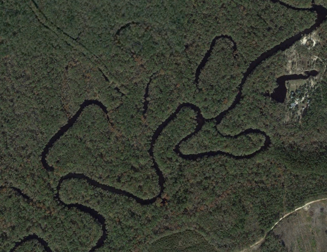
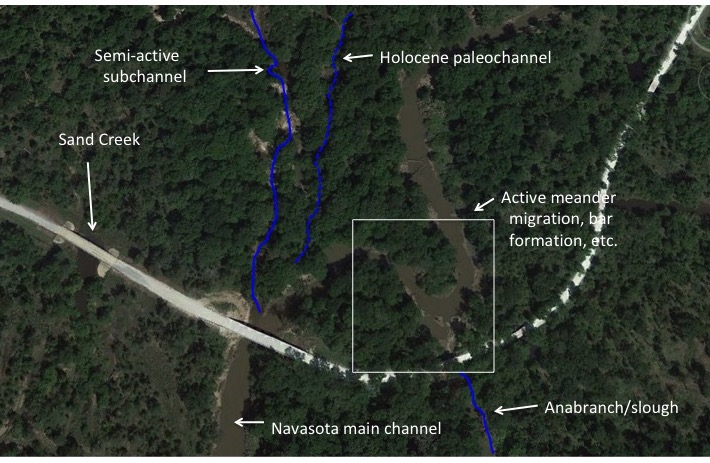
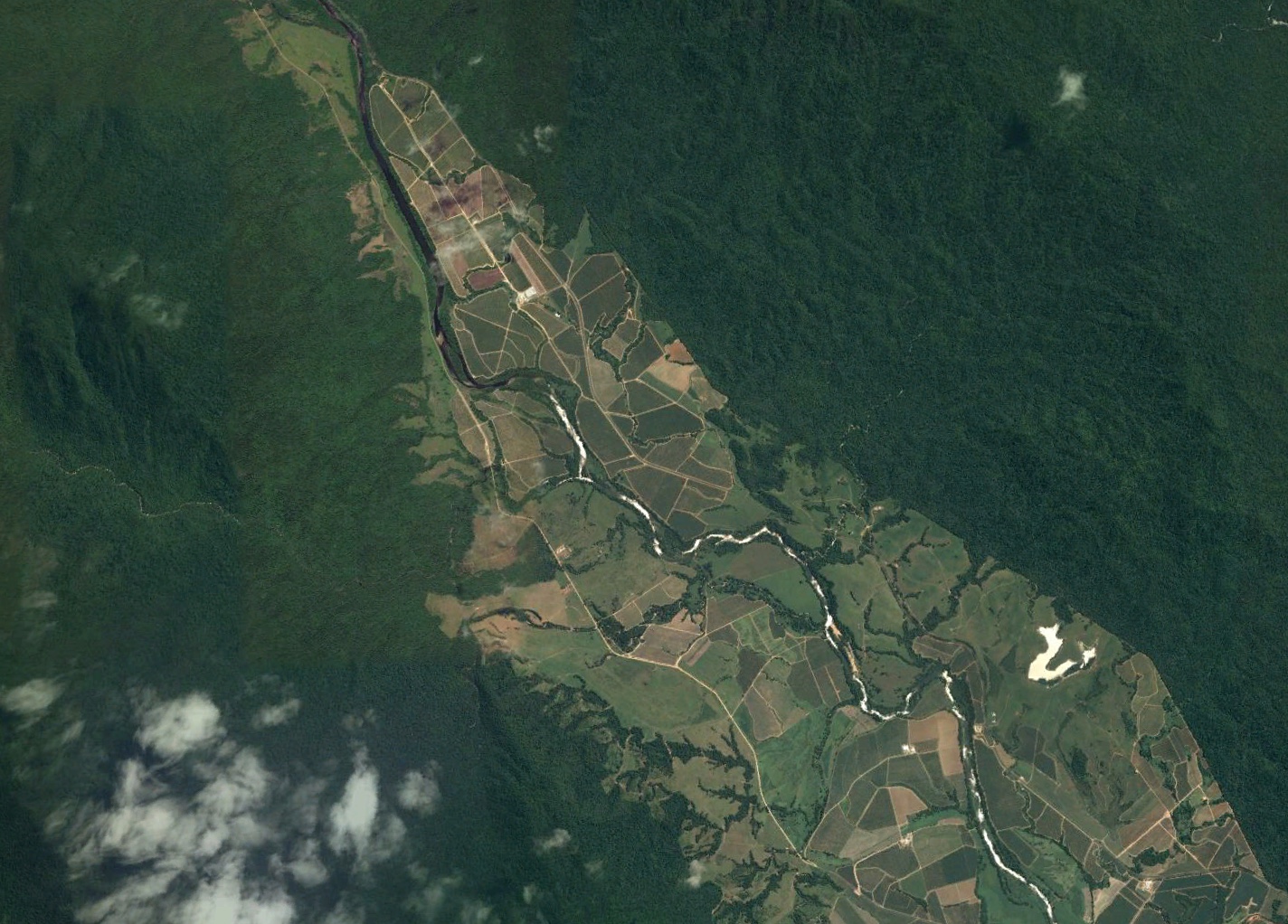
Those of us interested in effects of contemporary and near-future climate change on coastal plain rivers have focused, appropriately enough, on sea-level effects. Recent events suggest, however, that perhaps climate warming induced changes in the frequency, severity, and behavior of tropical cyclones (and other storms?) may be of comparable importance. Mega-rainfall events such as Hurricanes Harvey and Florence not only send a lot of water down the channel, but they do so via precipitation concentrated in the lower portion of the drainage basins. 

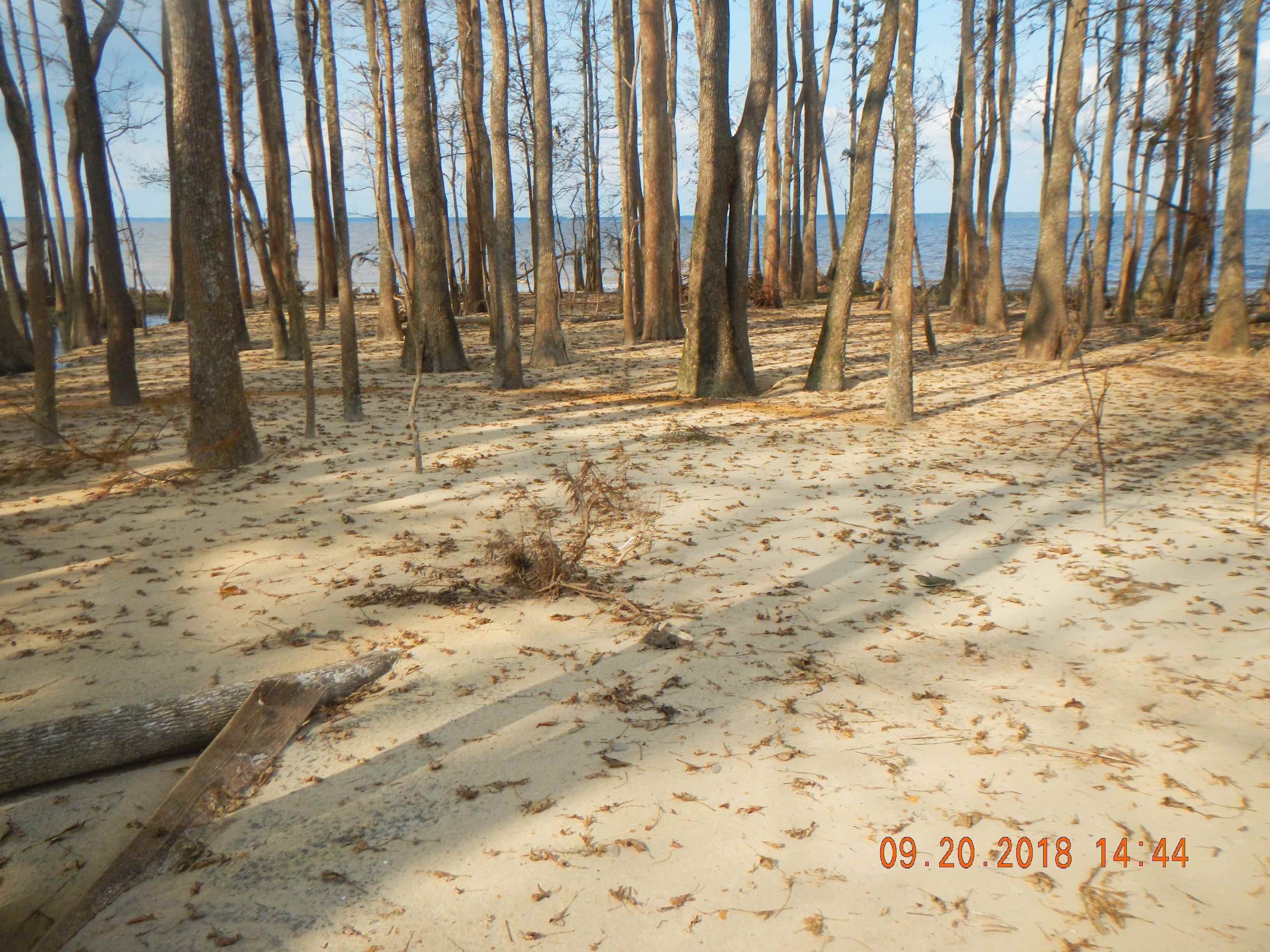
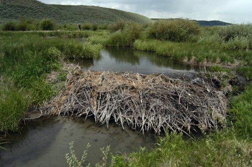
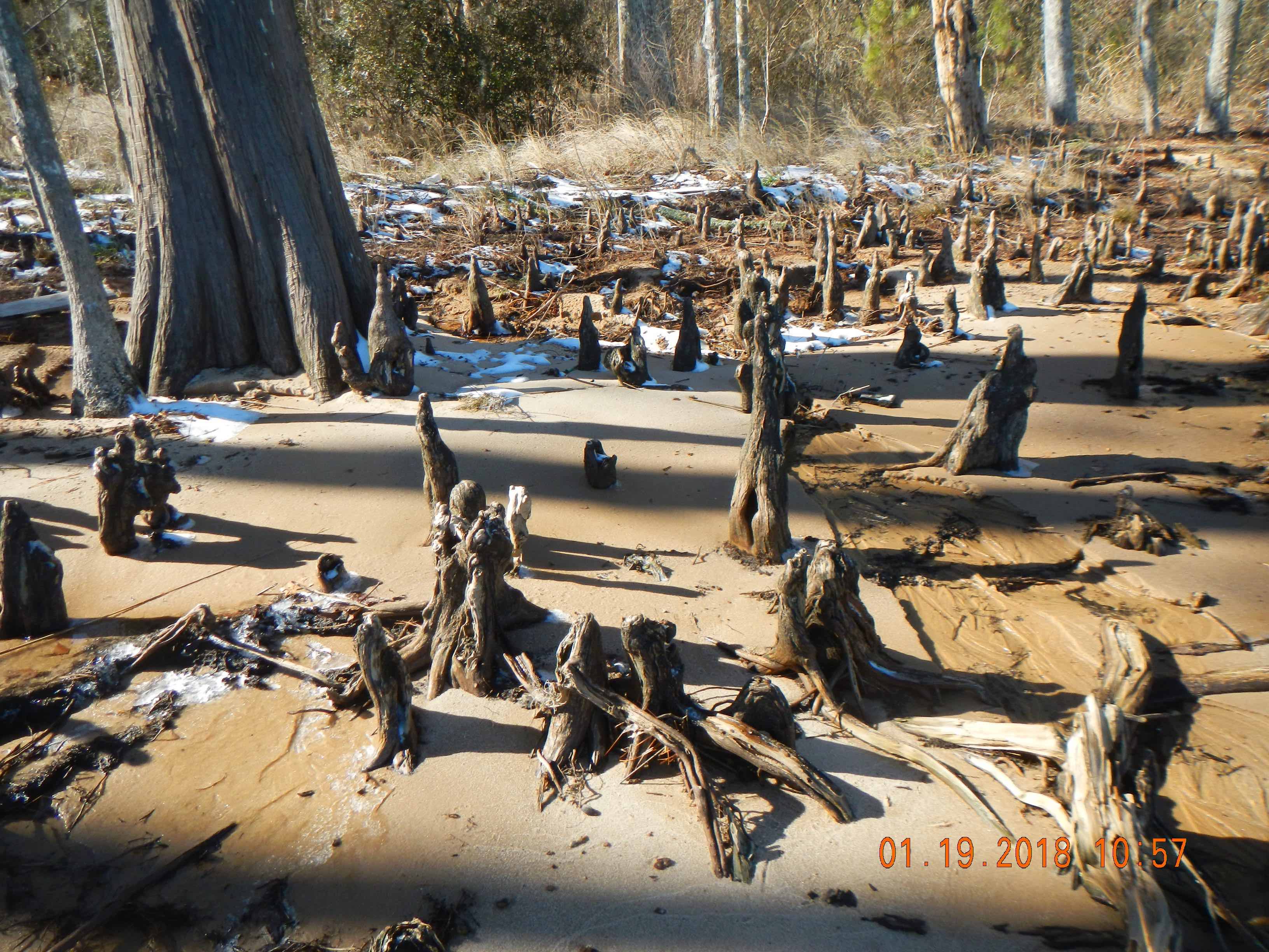
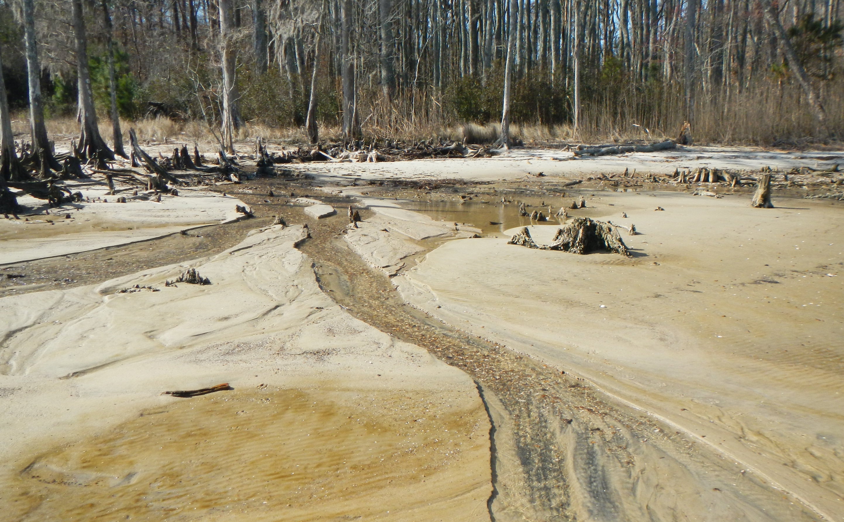
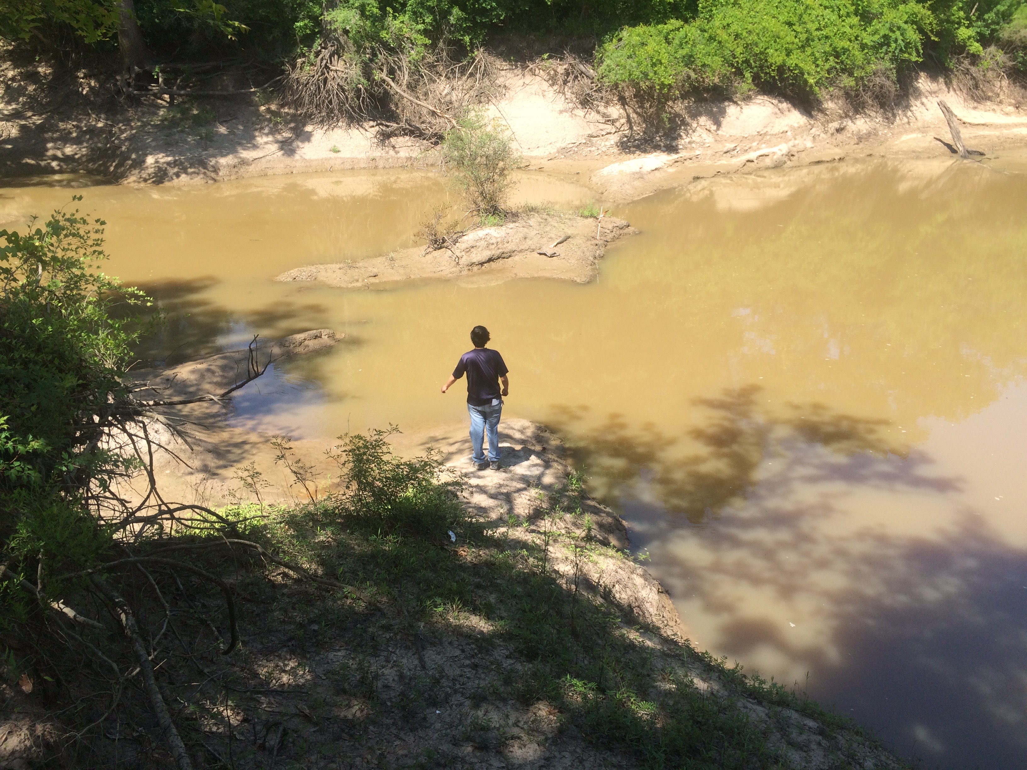
Cypress-Gum swamp near Croatan, NC covered with 0.5 m of sand during Florence. The pre-storm surface was organic muck. 

Posted 27 September 2018

A couple of years ago I blogged about generalized Darwinism in a post called Occam’s Selection. This is the idea that principles of variation, selection, and preservation or retention are applicable to development and evolution of many different phenomena. The GD label is most common in evolutionary economics, but the notion is constantly being reinvented in many different fields. 

A recent example is Selection for Gaia Across Multiple Scales, published in Trends in Ecology and Evolution. The issue is how biological natural selection, which operates at the level of individuals, could result in evolutionary trends at ecosystems and broader scales, including the self-regulating biotic/abiotic coupling of the global Earth system. 

It seems to be well established now that traditional natural selection can produce nutrient cycling and some degree of environmental regulation at local and ecosystem scales, an ideat hat was broached at least 30+ years ago by Charles Smith and well articulated in an explicitly Earth system science/Gaia theory context by Andrei Lapenis (2002). My own $0.02 worth (Phillips, 2008) showed that the only requirement of developmental trends toward, say, increasing diversity and productivity is that more efficient resource use confers some sort of survival and reproductive advantage. 

For any ecological system (such as this oxbow lake in southeast Texas) to show a trend toward increasing productivity over time, all that is required is biological saturation (all niches are eventually occupied) and the principle that more efficient resource use results in a survival or reproductive advantage. 

Some recent models point to a phenomenon of “sequential selection” for global environmental regulation, in which unstable outcomes are short-lived, and result in destruction and reorganization until a stable state is found. Thus repetitions of a system over time allow it to develop stabilizing mechanisms. While these specific models, applied to ecosystem and Earth system science, provide some new phenomenological insights, the fundamental idea that more resistant and resilient (dynamically stable) features tend to persist and recur while fragile and unstable ones are transient has been around awhile. 

In geomorphology the basic idea probably goes back much further, but a couple of examples whereby the term “selection” is explicitly applied to this phenomenon are Leopold (1994) and Twidale (2004).Nanson and Huang (2008) took these ideas a step further, showing how iterative adjustments (conceptually similar to sequential selection) result in “survival of the most stable” stream channel configurations.  Variations occur and selection happens in all sorts of phenomena and temptation is strong to propose natural laws or goal functions. For example, some variants of generalized Darwinism espouse a persistence principle; i.e., nature seeks persistent forms.  The "nature seeking" part is wholly unnecessary, however. A more accurate, if tautological, way to put it, is persistent forms persist. Thus they are more common and last longer than other forms. They are selected for, probabilistically (as almost all selection occurs), and their common occurrence is an emergent property of this selection, and do not require any goal functions on the part of Mother Nature.

In fact, I have come to view these phenomena as axiomatic. In a recent article (currently available online only) outlining axioms for interpreting natural landscapes, one of the axioms is expressed thusly: “Selection occurs. . . . Selection is a probabilistic notion that more stable, durable, and efficient features and phenomena are more likely to persist and be reinforced, relative to those that are less so. Thus, as the pathways and networks described above develop, they are strongly influenced by selection phenomena.”

Posted 3 September 2018

During some recent fieldwork doing forest biogeomorphology with colleagues in the Czech Republic, the idea of biogeomorphic equivalents came up. A biogeomorphic ecosystem engineer organism has a biogeomorphic equivalent if another species can potentially do the same biogeomorphic job. For example, bacteria that consume iron are important agents of weathering. There exist numerous species of iron-eating microbes, so if one is eliminated for whatever reason, another takes its place. Thus these Fe-processing bacteria have biogeomorphic equivalents.

Acidophilous iron-oxidizing bacteria (USGS photo).

On the other hand, there exists no biogeomorphic equivalent for the stream-damming effects of beavers. The disappearance of Castor canadensis from a landscape means the loss of their biogeomorphic effects, as no other organism (save humans, of course), dams up streams.

Wyoming beaver dam (photo: Wildlife Conservation Society).

The notion of equivalents raises a number of interesting questions for geomorphology, ecology, and environmental management. If an organism has no biogeomorphic equivalent, then its loss has implications well beyond the biological and ecological--and the same goes for the introduction of a new species. The reintroduction of beavers, for instance, has been used as a stream restoration tool, to partly reverse the effects of earlier beaver removal.

We also have to consider equivalency as a matter of degree, and with respect to particular effects. In some tidal freshwater rivers of the southeastern U.S., for example, sea-level rise is resulting in reduction of bald cypress and an increase in tupelo gum (aka water tupelo). The trees occupy similar ecological niches; both grow in swamps and along slow-moving streams and develop wide, buttressed trunks (they often grow together in the same habitat). There is, no doubt, some overlap in their biogeomorphic impacts, particularly with respect to sediment trapping and stabilization of riparian and wetland substrates. However, cypress develops subaerial root structures called "knees" that tupelo does not have. These knees have significant (though not well studied) effects on hydraulic roughness, and on resistance of banks and shorelines to erosion. Thus tupelo gum is only a partial biogeomorphic equivalent of cypress.

Cypress knees, Neuse River estuary shoreline, North Carolina.

In forests, tree species may have biogeomorphic equivalents with respect to slope stabilization and bioprotection, but not with respect to other factors. In the Czech forests where I was recently, for instance, various factors (climate, natural and human disturbances, succession, forest management) have resulted in the decline of beech and increase of Norway spruce (or vice versa).  These trees have fundamentally different impacts with respect to uprooting dynamics, root architecture (and phenotypic plasticity with respect to root adaptations to substrates), surface mounding and mass displacement, litter chemistry (which affects weathering), and production of stemwash and trunkwash.

Basal mounding and hummocky topoography created by Norway Sspruce, Jeliscky Mountains, Czech Republic.

It may also be useful to think about biogeomorphic functional groups.  Functional groups are fairly broadly and variously defined in ecology, but generally represent organisms--not necessarily genetically or evolutionarily related--that perform similar roles and functions in ecosystems.  For example, iron-oxidizing, calcite-precipitating, and sulfate-reducing bacteria would represent three biogeomorphic functional groups that are entirely consistent with functional groups in microbial ecology. On the other hand, I'd have more trouble arguing that there exists, say, a tree-uprooting functional group, as the same species might uproot or not depending on the environmental context.

Peat-forming mosses, for instance, could readily be defined as a biogeomorphic functional group. But what about, say, ants that build mounds? These are important biogeomorphic agents in many landscapes, but the set of mound-building ants includes those that build tiny mounds varying over several orders of magnitude in size, and mounds made entirely of mineral soil or vegetative matter, and lots in between.

These ants in the Sumava Mountains (Czech Republic/Germany) build large mounds, but almost entirely of spruce needles and plant litter rather than mineral soil.

By starting to think about biogeomorphic equivalents and functional groups, however, we can perhaps begin to frame the ever-expanding base of biogeomorphic knowledge in terms directly applicable to environmental management. We can also hopefully gain some new scientific insights. For example, the bacterial functional groups and biogeomorphic equivalents mentioned above all relate to "eating" or using particular resources--if one microbe is not going to consume the iron, then something else will. Peat-forming mosses occupy habitats that, if they don't utilize, something else will. By doing what they do, the bacteria will perform their biogeomorphic roles. By living and dying in anaerobic environments, the mosses are likely to form peat. By identifying common traits of biogeomorphic equivalents and functional groups (if any), we may be able to gain further insight into reciprocal interactions among landforms, surface processes, and biota.

--------------------------------------

26 July 2018

Some have argued that in geomorphology and physical geography the term "tipping point" does not describe any concepts or phenomena not long recognized by the fields. The tipping point concept does not (it is argued) have any conceptual or analytical value added. I agree. Here is a previous post on tipping point metaphors.

Blanco River, Texas.

Notwithstanding that, tipping point terminology is au courantin both public discourse and science, particularly as it relates to global and broad scale environmental change. Thus--perhaps analogously to buzzwords such as "sustainability" and "resilience"-- if you want to be a part of broader scientific conversations, it pays to employ the trendy term.

In 2016 at the European Geoscience Union meeting I was part of an organized session on tipping points. The goal was not to uncritically accept or to ratify the term or the concept, but to explore its potential utility in geomorphology. My paper in that session eventually resulted in the article below, just published. The motivation was that if we hope to recognize and respond to future tipping points (or whatever we choose to call them) we should make use of what we know about past TPs. I chose Texas rivers because of my own extensive experience working on them, and an extensive mass of work by others.

A preprint version is available here, and the final published version here.

___________________________________________________________

Posted 11 July 2018

Where forests grow on thin soils over bedrock, the effects of individual trees (as well as the effects of forest cover and litter) may work to deepen or thicken the soil. This occurs due to root penetration of bedrock joints and fractures. This in turn facilitates weathering and funnels moisture into the rock. Uprooting of trees may “mine” bedrock encircled by roots, and leave a locally thicker mound as rootwads deteriorate. If trees do not uproot, as stumps rot away the depressions—often extending deeper than surrounding soil—fill with soil, sediment, and organic matter. This thickening of the soil is a form of direct, positive ecosystem engineering in that it increases habitat suitability for the engineer organisms (the trees). 

Chinquapin Oak growing in limestone, Mercer County, Kentucky.

Eventually, however, the average soil or regolith thickness may increase such that tree roots no longer contact bedrock. Then the biogeomorphic ecosystem engineering effects of the trees on soil thickness ceases. In effect, you have self-limited biogeomorphic ecosystem engineering. 

Root groove associated with accelerated weathering along a root in sandstone, western Arkansas.

This phenomenon almost surely occurs with other organisms and environments, and with respect to trees and soil thickness, certainly occurs in non-karst environments. However, you have to start somewhere, and I started studying this phenomenon by looking at  self-limited biogeomorphic ecosystem engineering in epikarst soils in central Kentucky. The result, an article in Physical Geography so titled, was just published. The abstract is below. You can also get at it here.

Posted 28 June 2018

As sea level rises--and it is rising!--it is causing geomorphological, hydrological, and ecological changes in coastal environments. Though "bathtub" models, which show where the shoreline would be with sea level increased by a certain amount, are useful in showing areas of potential impact, that's not how actual responses to sea level work. Not only does the ocean level change, but also the base level for rivers and terrestrial processes, salinity, ecological habitats, hydroperiods, and any number of other factors. 

Sand and mud flats along the eroding Neuse River estuary shoreline, NC. 

As sea level rises we can generally expect changes along environmental gradients (from, e.g., lower, wetter, and saltier to higher, drier, and fresher) as these gradients are translated inland. However, there are multiple gradients involved, and interactions between, e.g., water chemistry, hydrological, geomorphic, and ecological gradients. Furthermore, there are often nested levels of gradients. For example, the fluvially dominated freshwater to tidally dominated saltwater gradient along a coastal plain river will encompass a number of tributaries with the same gradient, which themselves may have tributaries with the same gradient, etc. 

Thus, just as the effects of sea level rise are more complicated than simply filling a coastal bathtub, they are also more complicated than simple regional linear transitions of the type often featured in efforts to map vulnerability to sea level rise, sequence stratigraphy, and vegetation succession (to name a few examples). 

But, at least if we consider multiple environmental gradients, and the presence of spatially nested gradients, can we still understand effects of sea level rise based on those gradients? That was the main question in my latest published article,  Environmental gradients and complexity in coastal landscape response to sea level rise,  published in Catena169: 107-118(you can also access it here).

The abstract, and the answer to the question above, is shown below. 

This continues work I started a couple of years ago, returning to the coastal and coastal plain landscapes of eastern North Carolina, where I got my research start as a graduate student at East Carolina University (MA, 1982), and later with the Pamlico-Tar River Foundation of Washington, NC (1984-6), and as a faculty member at ECU (1988-1997). 

Earlier this year,  Coastal wetlands, sea level, and the dimensions of geomorphic resilience  was published in Geomorphology 305: 173-184 (also here).  That study, based on detailed analysis of a couple of small wetland sites, was concerned with whether the coastal wetlands in question are dynamically stable (= resilient) to rising sea-level. 

The abstract is below: 

Osprey nest, Slocum Creek, NC. 

-----------------------------------------------------------

Posted 25 June 2018

This post continues a series exploring the idea of evolutionary creativity in Earth Surface systems (ESS). Previous posts introduce the evolutionary creativityconcept, explore the possibility of algorithmic evolution modelsof ESS, and discuss the appearance over time of new varieties of landforms. 

-------------------------------------------------------------------------------------------------------

Biologists have put a great deal of effort into identifying the variety of life forms. While there is only one extant species of the genus Homoand 11 of Canis, there are more than 600 species of Quercus (oak trees) and >350,000 of beetles (and counting).  

British biologist J.B.S. Haldane, when asked what he had learned of the Creator from his studies, is supposed to have answered that the Creator has "an inordinate fondness for beetles" (or words to that effect). (Photo: Cincinnatizoo.org). 

ESS are at a higher level of aggregation, such that soil types, landforms, etc. are more commensurate with, say, biological communities than with species or other biological taxonomic levels. Still, we have put a lot less effort into cataloging variety of ESS. More than a century soil classification and mapping, for instance, has so far identified <20,000 different soil types (series) in the USA. 

Landforms are classified in even less detail than soils (note that there exists no generally accepted scheme of geomorphic taxonomy or landform mapping). Even a treatise on aeolian geomorphology, for instance, will recognize perhaps a couple of dozen types of sand dunes, while even my limited observations suggest that the variety--considering sizes, shapes, activity, behavior, composition, soil & vegetation development, subsidiary features, etc.--is pretty much limitless. This, of course, hampers any effort to assess the appearance of new varieties.  

The level of classification detail varies in different areas of geomorphology. For example, some stream channel classifications are very detailed--at least compared to those for other landforms. Still, even for stream channels the level of detail is orders of magnitude less than that for soil taxonomy, which is far less than for biota. 

So I did a little thought experiment with respect to dolines. Dolines are karst sinkholes. As far as I can tell, geomorphologists recognize just four to six basic types, depending on whether they are formed primarily by dissolution from the top down, or collapse into a subsurface dissolutional cavity, and whether there exists a layer of regolith overlying the dissolving rock or not. 

Dolines overlying Hang Son Doong cave, Vietnam (https://en.wikipedia.org/wiki/File:Son_Doong_Cave_Doline_with_Scale.jpg)

Solutional doline, Slovenia (photo: Matej Gabrovec)

I did this experiment using two guiding principles. First, before you can have dolines you must have karst, and before you have karst you have to have carbonate rocks. Carbonate rocks cannot form until the appearance of calcium-precipitating and concentrating organisms. Second, there has to be a first time for everything. That is, the contemporary range of karst features cannot have appeared simultaneously. The result is the figure below. 

The upper part, from the top of the figure down to "karst," can be viewed as chronological, according to the first guiding principle above. Beyond that, it identifies some of the variation that occurs, focusing on the dolines I'm most familiar with in Kentucky--regolith covered, collapse-type, drained by karst conduits, roughly circular in planform, and often connected to each other by underlying conduits or cave systems. The fat arrows in the diagram show many other pathways that could be followed, leading to many more types of dolines (and other karst landforms). The bottom line indicates someof the other significant ways dolines can differ. How many possibilities are there, even for collapse dolines? I don't know, but--a lot!

Collapse dolines in central Kentucky. 

Paleokarst appears in the geologic record from the early Proterozoic, roughly two billion years ago. From that time, whatever the first karst landforms were have diversified into what we have at present (though some types may have gone extinct). This thought experiment for dolines--and the same could no doubt be done for sand dunes, solifluction lobes, oxbow lakes, or any number of features--convinces me, at least, that "creativity" has occurred (and is occurring) in the evolution of landforms and other Earth Surface Systems. 

Ik Kil Cenote, a doline in Mexico (www.worldfortravel.com)

-----------------------------------------------------------------------------------------------------------------------------------------

Posted 12 June 2018

This continues a discussion that started by considering the possibility of evolutionary creativity in landscapes and continued by exploring the possibility of algorithmic evolution models of Earth surface systems (ESS). 

In biological evolution by natural selection, new varieties arise via genetic mutations. Occasionally one of these turns out to be advantageous--the fitness of the organism is increased, and the variation is "selected" (recall that Darwin used natural selection to contrast with selective breeding of animals and plants by humans). The selected organism can reproduce, and pass the selected trait to its progeny.

Except to the extent that biota are part of them, ESS cannot reproduce, and do not have programs (i.e. genes) to pass along traits, good, bad, or indifferent. Landforms are a type of ESS that may (rarely) be abiotic, or more commonly, exist independently of organisms. Both organisms and landforms can producenew forms--through mutations in the case of biota, and via geomorphic transformations in the case of landforms. For instance, fluvial incision can produce terraces from floodplains, and long-term erosion produce valleys from anticlinal ridges. In some senses geomorphic change can be thought of as the production of new forms via transformations of earlier ones. 

Both biota and landforms can also propagate or expand their spatial coverage independently of size increases of individual organisms or landforms. This is most apparent with respect to the spread of, e.g., certain types or vegetation or microbes. Landforms may propagate over large areas by the growth of individual features (e.g., deltas, fans, floodplains), but may also propagate by the expansion of certain modes of landform development (e.g., badland erosion, channel network expansion, aeolian and fluvial bedform propagation). 

Badland erosion, Badlands National Park, South Dakota (Kevin Walsh photo). 

Landforms and organisms can both die--literally in the latter case and by being erased or obliterated in the former. Only organisms, however, mustdie over timescales of a few centuries or less. Landforms have the possibility of persistencebeyond the lifespan of any organism. 

Although there is no direct mechanism analogous to genes for passing on new landform traits, new varieties of landform can be produced. There exist at least four geomorphological analogs to mutation: biological mutation effects via biogeomorphology, geological inheritance, local disturbances, and contingency. 

Few landforms are truly abiotic, and many are strongly influenced by biological and ecological processes. When successful biological mutations occur, and the organisms have biogeomorphic ecosystem engineering effects or are bioconstructors of landforms, biological speciation can be associated with the appearance of new landforms (the example of meandering rivers was given in the previous post). The evolutionary appearance of, e.g., calcite-secreting cyanobacteria, coral organisms, and termites resulted in the appearance of stromatolites, coral reefs, and termite mounds. 

Biogenic weathering, South Bohemia, Czech Republic.

Mutations are perturbations of existing genes, so it may be hard to see how geological inheritance can be analogous. First, consider geological effects on landforms. Even within a given lithology, no two (e.g.) sandstone or granite geological formations are identical--that's why formations are given local and regional names. Within these formations a great deal of structural and lithological variation occurs, which often profoundly influences topography and morphology. Second, consider that "inheritance" can occur from relatively abrupt geological perturbations--volcanic eruptions, earthquakes, tsunamis, for instance. Third, note that inherited geological variations appear--sometimes very gradually, sometimes suddenly--as geomorphological denudation occurs, exposing new materials and structural features. 

Structurally controlled weathering near Zlin, Czech Republic. 

Another geomorphological analog of mutations may occur in the form of other local disturbances that may result in new varieties of landform. Human impacts (if you consider us separate from other biota) are one example; others may include storms, floods, and fires. 

Local disturbance--fire--created these unique landforms: Posthole-type stump pits with sealed pit walls (Sumter National Forest, South Carolina). 

Contingency as a source of variety refers to the fact that landforms and other ESS have irreducible elements of historical and geographical contingency. That is, no two places or environments have the same combination of environmental controls or influences, or the same history of changes and disturbances. These unique, idiosyncratic aspects of ESS consistently produce new varieties of landform, particularly if we endeavor to describe or designate landforms with greater specificity than just, say, doline or scree slope. 

Though ferricretes--and probably "ferricrete hash" similar to this--occur elsewhere, the "perfect" combination of topography, drainage patterns, geochemistry, fossiliferous cemented material, and erosional exposure of zones of iron accumulation results in this unique feature along the Neuse River estuary, North Carolina. 

--------------------------

Posted 10 May 2018

This post is a continuation of a thread that starts here.

The algorithmic evolution models pioneered by Gregory Chaitin (see Proving Darwin,2012 for a very readable introduction) are based on a metaphor of an organism as a K-bit program that takes the original organism A and produces a mutated organism A'. The fitness of the organism/algorithm is measured by the largest integer the algorithm can calculate. Thus a mutation that increases the largest calculable number is retained, while others are rejected. This continues until BB(N), defined as the largest integer that can be produced by a <N-bit program that produces a single integer and then halts. 

This is a plausible analog for biological evolution, in which continuous improvement in fitness is possible, up to some maximum limit. In nature the maximum limits are presumably associated with maximum rates of biological processes rather than algorithmic complexity and information (i.e., BB(N), which has the awesome name of the Busy Beaver Number). 

Busy beavers--a myth perhaps, but a useful metaphor (The Far Side, by Gary Larson).

But can we make analogous arguments or models for, say, hillslopes or channel networks or ecosystems? What is an appropriate measure of fitness (in a real or metaphorical sense) in Earth surface systems (ESS)? A number of hypotheses have been proposed for optimal structures and configurations of, e.g., ecosystems, channel networks, topography, etc. These are reviewed here, where I also argue that most, if not all of these principles can be reduced to (or subsumed under) the idea of efficiency selection--more efficient forms are more likely to persist and grow or occur repeatedly than less efficient ones.  I have also discussed why maximum efficiency forms are not observed in nature quite as often as you'd think (Part 1, 2,3).

One argument that might be made against ever-increasing fitness or efficiency in ESS is that these were achieved early on--that is, the very earliest flow networks, for instance, were capable of developing optimal forms, even if not all did. No evidence exists of increasing variety over time as with biota--right? Well, not quite. Evidence from paleohydrology and the rock record, for instance, indicates that (except perhaps in a few situations with fine-grained cohesive soils), all rivers were braided until vascular plants and woody vegetation came on the scene. Then meandering and anastamosing forms--new ways of achieving maximum efficiency--developed. These studies are backed up by both numerical modeling and laboratory experiments, by the way. Thus creativity and innovation in biological evolution was accompanied by creativity and innovation in fluvial systems. 

Meandering rivers (this Google Earth example is the Waccamaw River, South Carolina) did not come on the scene until vascular plants evolved, increasing bank stability. 

Another key point is that in many cases optimal or maximum efficiency states in ESS are non-singular--that is, there is more than one way to achieve a given state. For example, we've known for nearly 30 yearsthat maximum efficiency configurations in stream channels can be achieved with an essentially infinite combination of quantitative values of width, depth, velocity, slope, and roughness, and even with multiple possible qualitative combinations of increases, decreases, or no change in the key hydraulic variables. Similarly, "optimal" forms of food webs or flow networks may be statistically similar or identical, but the specifics are highly variable. 

If we think of ESS as individuals rather than categories--i.e., the Little Pee Dee River channel network rather than "alluvial channel networks"--then it is plausible that individual ESS might, through various changes, "creatively" produce ever more efficient variations until maximum efficiency is reached. 

This micro-delta (Moccasin Creek, NC) has multiple degrees of freedom to adjust its configuration. 

This in turn suggests that algorithmic evolution models may be applicable to ESS. But there are other key differences among biological, physical, and biophysical systems to consider. More about that in future posts.

----------------------------

Posted 4 May 2018

Recently I had the pleasure of visiting the geography department at Texas A&M, and during my trip I was able to revisit some field sites along the Navasota River I had last been to in 2006. The lower Navasota is basically an anastamosing system--there is a single dominant channel, but multiple subchannels, some active at normal and low flows, at any given valley cross-section. One place is particular, Democrat Crossing, is a particularly confusing locus of recent and ongoing channel change. 

2017 Google Earth^TMimage of Democrat Crossing. Sand Creek is actually a perennial or active Navasota River subchannel (semi-active means, in my lingo, that it usually carries flow, but may dry up in low-flow periods). Some of the subchannels have been highlighted with blue lines I added, as you can't really see them if you don't already know they are there. 

This reminded me of the fact that in a number of rivers in many locations, I have noticed hotspots of lateral channel change. I began at one point (in 2013) to write up a paper/proposal to study this phenomenon, but it got lost in the shuffle. I present it below, in its quite incomplete and preliminary form, in the hopes that someone else may be inspired. 

I visited the Navasota sites with Dr. Inci Guneralp and her PhD students Cesar Castillo and Billy Hales. I am confident they will have this particular hotspot figured out soon!

Introduction--Hotspots of lateral channel change

Hotspots of lateral channel change are specific reaches or subreaches where channel migration, cutoffs, avulsions, and other changes are more evident, frequent, and active than in upstream or downstream reaches. The purpose of this paper* is to examine the phenomenon of lateral change hotspots to identify the causes of this localized activity, and how these hotspots relate to the evolution and environmental controls of fluvial systems. 

Examples of lateral migration hotspots are shown in Figure 1**. While these are rather obvious cases, as a starting point hotspots can be defined as areas of significantly greater sinuosity than up- or and downstream reaches, and/or with evidence of more frequent or recent cutoffs, oxbows, meander scars, multiple channels, paleochannels, or islands (collectively referred to as channel change indicators; CCI). As a rule of thumb, hotspots have sinuosities at least 30% greater, and/or a density of CCI at least double that of  up- or downstream reaches. 

Figure 1.  Tully River, NE Queensland, Australia. The Tully emerges from a confined valley, and immediately begins laterally migrating (note all the sand point and lateral bars, absent in the confined reach) and avulsing (note several abandoned channels and high-flow anabranches). (Google Earth^TMimage). 

Understanding hotspots of lateral channel change can shed light on channel change more generally. The hotspot concept is directly relevant to river planforms, sinuosity, cutoffs, avulsions, and lateral migration. These are also related to slope and vertical adjustments in several ways. First, increases in sinuosity are often a direct response to a local increase in slope, e.g., due to tectonics or base level change (Schumm, 2005). While sinuosity is defined as the ratio of length along the main channel or thalweg divided by valley distance, it is also the ratio of valley slope to channel slope. Further, crevasse, avulsion, and cutoff phenomena are associated with vertical changes such as channel aggradation (Jones and Schumm, 1999; Slingerland and Smith, 2004). 

Localized increases in lateral activity are presumably linked to changes or variations in boundary conditions or controls along a river, or to local perturbations. Since these hotspots are relatively easy (at least as compared to other aspects of fluvial geomorphology) to identify from maps and imagery, they are potentially an important tool for indentifying critical hinge points, boundaries, and localized disturbances. Additionally, lateral channel change hotspots are associated with higher levels of geodiversity and hydrodiversity, and thus are likely candidates to be local hotpots of habitat, soil, and biodiversity. Finally, lateral change hotspots may often be associated with erosion and flood hazards, land loss, and a variety of river and riparian management and engineering issues. 

Theory and background

Lateral channel change requires bank erosion on at least one side of a channel, or a levee or banktop breach (crevasse) that results in a new channel. Thus for such changes to occur the force of flow, as directly measured by shear stress, or indicated by stream power, must be greater than the resistance of bank or floodplain materials. Thus, hotspots may be due to local factors that increase the force/resistance ratio. 

Thus, local increases in flow (discharge and/or depth) and/or slope can increase the force/resistance ratio. This can occur due to hydrologic inputs, geological or tectonically imposed channel slopes, or flow constrictions, which may increase depths and velocities and create steeper hydraulic slopes. 

Force/resistance may also be increased due to lower resistance, often associated with low-cohesion but relatively small grain size materials (i.e., sand or gravel), or reductions in vegetation cover. 

Stream power and shear stress are also related to sediment transport capacity and competence, and channel change can also be associated with changes in the relationship between sediment supply and transport capacity (SS/TC). This may work in several ways:

•A sharp decrease in SS/TC (e.g., below a dam) may result in flow with excess force. While this most often results in vertical scour, where the latter is limited by resistant bed materials or local base levels, increased lateral migration may result.

•A significant increase in SS/TC may trigger a change from a single-channel to an anabranching planform (braided, wandering, or anastamosing). 

•Channel aggradation associated with SS/TC > 1 is a setup condition for cutoffs and avulsions. 

While this could be triggered by flow losses or diversions, the most likely causes are reduced slope (thus lowering TC), or major inputs of sediment, e.g., from slope failures or tributaries. Flow obstructions such as large woody debris, or damming by ice, landslides, migrating aeolian dunes, etc., can also lower hydraulic slopes and reduce flows. 

Finally, lateral migration may be a simple function of lateral accommodation space—that is, room to move. Valley confinement (see Brierley and Fryirs, 2005) and valley-to-channel width ratios are important in this regard. Lateral migration hotspots could be controlled by local variations in valley width. 

(there was some additional musing & arm-waving about methods, but that's pretty much it).

Navasota River at Democrat Crossing. There are no obvious external controls here (e.g., valley width/confinement; evidence of tectonics or listric faulting, large sediment inputs, etc.). 

*As mentioned, no paper ever actually materialized.

**There would have been more than the one example shown; they are not that hard to find. 

--------------------------

Posted 2 May 2018