In my own work on pedology, soil geography, and soil geomorphology, there are at least three overlapping concepts of soil memory (or pedological memory) that at least generally, if clumsily, parallel the pedological literature as a whole.  

One is based on the fundamental idea of soils as products of the environment, reflecting the combined, interacting influences of geological (or other) parent material, hydrological and geomorphological processes, climate, biota, all changing over time, and affecting each other and affected by the soil itself.  This is the factorial or state factor model of soils going back to Dokuchaev and Jenny, and the conceptual basis of soil geography, surveying and mapping. Inverting the logic—soils as evidence of the environment rather than the environment as an explainer of soils—is the basis of paleopedology and paleoenvironmental interpretations of paleosols. This concept of soil memory is that soils “remember” the environmental factors influencing their genesis and development.

Carsten Lorz has used the memory of soils such as this one in Saxony, Germany, to reconstruct Quaternary pedogenesis. 

A second soil memory concept is that of the soil as a container for historical evidence and artifacts. This can be independent of the factorial model in that soils may contain fossils, archaeological artifacts, pollen, charcoal, trash, and pollutants that are unrelated to the factors or soil formation, or whose interpretation does not require an understanding of their pedogenetic impacts. Thus the soil “remembers” specific events and episodes that happened on or in it. 

Krotovinas and other biotic traces in an eastern North Carolina soil. 

A third concept is related to dynamical instability and deterministic chaos. When, as is not uncommon, soil development is characterized by instability and chaos (equivalent in many cases), small changes and disturbances may have impacts that are disproportionately large and long-lived. Thus a soil can “remember” effects of, e.g., a tree that once grew, an ant mound that was once constructed, or an erosional event that once occurred long after direct evidence of the tree, ants, or erosion is long gone.

A void created by the recent death and decomposition of a pine tree in eastern North Carolina. Pedologic impacts of the tree may well be evident long after all evidence of the tree—including this void, which will be infilled—are gone. 

This got me to thinking about soil memory metaphors. 

Soils as Text

Fill-in-the-blank as text is a common metaphor in the critical and postmodern social sciences, and is not necessarily rare in the geosciences, either.  This metaphor is applicable where soils represent not just a container for artifacts or a particular piece of evidence, but a more comprehensive record of environmental change, enabling those who can read the text to tell a story. 

The soil-as-text analog may thus apply to the use of soils or paleosols as (paleo)environmental indicators and tools for environmental reconstruction. Soils as geomorphological, hydrological, and ecological indicators—for example in wetland identification—also reflect soils as texts. 

Rocks of three distinctly different lithologies from a single soil pit in Podyii National Park, Czech Republic. These, along with other aspects of the soil, could tell a story if we can interpret the text—perhaps some ancient humans rounding up rocks for a fire pit?

Soils as Archives

How does an archive differ from a text? A text contains at least fragments of a story or narrative, while an archive is a container or repository. This metaphor thus applies to the “container” concept of soil memory, whereby soils or paleosols are host media (archives) for fossils, pollen, charcoals, artifacts, phytoliths, biochemical markers, and so on. 

Root traces in the subsoil from upstate South Carolina. 

Soil Palimpsests

A palimpsest is a manuscript or piece of writing material on which the original writing has been effaced to make room for later writing but of which traces remain—think back to the days of papyrus scrolls, or erasures and write-overs in your fieldbook, though we were all told to cross out and never erase. 

Landscapes as palimpsests is a pretty well known, and very apt, metaphor in geomorphology. Landforms and topography often represent not only the most recent “writing” of geomorphic processes and environmental control, but traces of past writings (or texts!) as well. 

The metaphor is apt for soils as partial, censored paleoenvironmental indicators for multiple episodes and environments—entirely consistent with the pedological concept of polygenesis. The palimpsest metaphor is also useful when thinking of soils or  landscapes as incomplete indicators of multiple episodes of environmental changeor disturbance events.

An alluvial soil in the Sumava Mountains, Czech Republic. The pedological and sedimentological archive are combined in this case. The stratigraphy records a standard alluvial fining-upwards sequence, while the horizon Pavel Danek is pointing to records the influence of podsolization processes. 

Seat Cushion Soils

In soil hydrology and soil mechanics a “seat cushion” metaphor of soil memory has been invoked. When you sit for awhile and get up—especially when you’re a big ol’ boy like me—your butt-print remains for a time, until the material can rebound and expand back to its original shape. This metaphor has been applied to relatively short-term soil memory, such as recovering the soil moisture memory of wetting events, or the soil mechanical memory of the removal of imposed loads. 

Butterflies & Bailey Effects

Early work on chaos theory in atmospheric dynamics used the hypothetical case of a butterfly flapping its wings setting off a chain of dynamically unstable, chaotic changes that result in a tornado thousands of kilometers away (the first usage, as far as I can tell, is in a paper given by Edward Lorenz called “Does the Flapping of a Butterfly’s Wings in Brazil Cause a Tornado in Texas?”).  This, plus the fact that the famous Lorenz Attractor diagram looks a bit like a butterfly quickly made butterfly effects a general metaphor in chaos theory for small changes and variations having much larger outcomes and impacts. 

Bailey effects are named for the character George Bailey, in Frank Capra’s 1946 film (story by Philip Van Doren Stern) It’s a Wonderful Life.In despair, Bailey attempts suicide after a run of bad luck, in the belief that his life has not been productive or worthwhile, and is rescued by a guardian angel. Bailey is given the opportunity to see what his community would be like if he had never been born. The point is that the seemingly small, insignificant actions of a single person may have ripple effects and chain reactions that produce dramatically different outcomes. The Bailey Effect is a metaphor for a type of interconnection based on dynamical instability and conditionality. Stephen Jay Gould (1990) invoked the same metaphor in discussing contingency in biological evolution; his book is called Wonderful Lifein a direct nod to the film. 

To the extent soils are characterized by divergent development, conditionality, and path dependence in soil development, the butterfly and Bailey metaphors may be apt.  However, this kind of soil memory is unlike the others in that all evidence of the “remembered” conditions or events may be long gone or undetectably small. 

The short-range spatial variability in soil morphology shown in these soils along the Neuse River estuary (NC) reflect the effects of divergent pedogenesis associated with instability and chaos. 

Other concepts of soil memory and appropriate metaphors thereof are no doubt possible, if not already in print somewhere.  For me, at least, thinking of what soils may remember, how they recall it, and what stories may be told is the most useful way of tying soils to landscape and ecosystem evolution. 

Posted 12 March 2021

Questions or comments?  jdp@uky.edu

Off-road vehicle trails, especially those used extensively by ATVs (all terrain vehicles, four-wheelers, quads), are notorious for producing a lot of soil erosion. Over a period of several years, I was involved in a project funded by the U.S. Forest Service, to determine where the soil eroded from trails in the Wolf Pen Gap ATV trail system in the Ouachita National Forest, Arkansas was going. That the trails are eroding was never in question--the questions were how much and how fast, what the off-trail impacts on streams are, and where the eroded sediment goes.

Sediment-laden runoff from an ATV trail in the Wolf Pen Gap complex near Mena, Arkansas.

The last of a series of articles based on this work has finally been published, as shown below!

This was actually the second-to-last that we produced, but it took longer to get published. The last one was in print last year:

My co-authors in these two were Dan Marion, recently retired as a research hydrologist for the USFS (and an adjunct professor at Kentucky), and Katie Kilcoyne, a UK graduate who at the time we did this work was a geography major at Kentucky. 

A complete bibliography of our work over the years on the ATV trails is below. Authors marked with asterisks were University of Kentucky students at the time the articles were submitted:

Marion, D.A., Phillips, J.D., Yocum, C., *Jahnz, J., 2019. Sediment availability and off-highway vehicle trails in the Ouachita Mountains, USA. Journal of the American Water Resources Association https://doi.org/10.1111/1752-1688.12793.  

Phillips, J.D., Marion, D.A., *Kilcoyne, K. 2021. Fine sediment storage in an eroding forest trail system. Physical Geography 42, 50-72. https://doi.org/10.1080/02723646.2020.1743613. (attached) 

Phillips, J.D., Marion, D.A., *Kilcoyne, K. 2020. Concentration and divergence of sediment in an erosional landscape. Geomorphology 367: 107281. 

Marion, D.A., Phillips, J.D., Yocum, C., *Mehlhope, S.H., 2014. Stream channel responses and soil loss at off-highway vehicle stream crossings in the Ouachita National Forest. Geomorphology216: 40-52. 

Phillips, J.D., Marion, D.A., 2019. Coarse sediment storage and connectivity and off-highway vehicle use, Board Camp Creek, Arkansas. Geomorphology 344: 99-112.

Questions/comments: jdp@uky.edu

Posted 18 February 2021

Every geomorphologist, soil scientist, farmer, backhoe operator or other person who digs holes in certain areas is familiar with them—floaters. I am not sure how widespread the terminology is, but the phenomenon is ubiquitous in areas where the regolith is derived mainly from underlying bedrock. Floaters are large rock fragments, unattached to underlying bedrock, within a soil or weathering profile.

Floaters in a limestone weathering profile, central Kentucky.

For farmers and excavators, floaters are mainly an annoyance. For pedologists and geomorphologists they can also be an annoyance. This is not only due to the difficulties they pose for digging and sampling, but because—particularly with augers, probes, and core samplers—they can easily be mistaken for underlying bedrock, resulting in underestimates of the depth and thickness of soils, regoliths, and weathering profiles.

But can these floaters tell us anything about weathering profile, critical zone, and regolith evolution?

My unofficial definition of a floater is an isolated rock fragment of roughly boulder size or larger (diameter of 256 mm or a little more than 10 inches). Smaller ones can generally—though not always—be nudged aside or at least moved a bit by a soil auger (my auger has a 100 mm or 4 inch diameter).  This lets you know, even when you can’t see them, that you haven’t yet hit bedrock.

I am also concerned here with floaters in situations where at least the lower part of the regolith is derived mainly from weathering of underlying rock, as opposed to, say, glacial till or debris flow deposits.

This soil, in the western Carpathian Mountains, Czech Republic, formed in landslide deposits. The floaters in this profile are not the sort I am concerned with here.

If we set aside cases where the parent material already contains large rock fragments (glacial drift, mass wasting deposits, debris flows, mine spoils, etc.), there are two general sources for floaters—the underlying bedrock, and upslope.

Bedrock

Rock weathers unevenly, particular by chemical weathering processes. Water follows preferential flow pathways into the rock along joints, fractures, etc., and water persists in certain physical settings within the rock. Weathering also tends to be self-reinforcing, often enhancing the variability in weathering. This can result in the persistence of unweathered or minimally weathered parent rock within a matrix of unconsolidated, weathered material. Some geomorphologists call these corestones, which is fine by me, but be aware that to some, corestone refers to a particular type of rounded rock formed by exfoliation weathering in granite.

Remnant unweathered rock  left behind as the weathering front moves downward can also result from situations where more resistant rock is interlayered with less resistant, more easily weathered lithologies. Sandstone and shale in sedimentary sequences are often interlayered, for example, as in flysch and other settings.  Rock decomposition may bypass the more resistant rock as the less resistant stuff is converted to saprolite or soil.

Minimally weathered bedrock remnants in a granite weathering profile in Union County, South Carolina.

Easily-weathered claystone separates more resistant limestone layers in Comal County, Texas.

These corestones (or whatever you wish to call ‘em) are in their original location in the weathered rock mass, and have not been transported. But corestones, and bedrock from the weathering front, can be transported vertically (as well as laterally) within the regolith. Downward movement can occur due to gravitational settling, undermining by faunalturbation (digging and tunneling by insects, earthworms, mammals, etc.), and undermining by subsurface erosional processes such as sapping and pipe erosion.

Corestones can also be moved upward. Tree uprooting is the single most common cause in forested settings, and most likely in general. Rock fragments are often uplifted as part of the rootwad, and settle into uproot pits or on the surface at higher elevations than they came from.  Freeze-thaw processes can move rock fragments upwards. Faunal excavation can obviously do so, too—most notably by Homo sapiens, but also by other species.

Black bear den in North America, showing large rock fragments excavated by the bear (bear.org).

Elephant digging soil and rock fragments in India (Rumble.com).

Uprooting of trees rooted in soil with floaters, or in substrate including transported rock fragments, can move the rocks upward. In addition, tree roots can penetrate bedrock, and remove previously unattached fragments –a phenomenon called bedrock mining.

Top: Root wad of uprooted Norway spruce in the Sumava Mountains along the Czech-German border. Rock fragments may be from glacial or periglacial debris rather than plucked from bedrock. Middle, bottom: Uprooted shortleaf pines from the Ouachita Mountains, Arkansas. Intact bedding shows that these were mined from bedrock. The shale (middle) is rapidly weathering, and the bedding will not be evident long. The uprooted sandstone bedrock (bottom) will persist.

Transported floaters

Rock fragments can be transported to a site, and work their way downward, by the processes referred to above.  Note that here I am referring to clasts transported to areas where the regolith is formed mainly by weathering of underlying bedrock, as opposed to colluvial or alluvial parent materials containing rock fragments.

Transportation in the post-industrial era may involve a number of mining, construction, and landscaping activities. Even earlier, though, humans (alone or with assistance from draft animals) transported stone for building structures and creating hearths and fire pits.  

In other cases, the main source is transport from upslope. Even where rapid mass wasting events (e.g., debris flows, avalanches, landslides, etc.) have not occurred, rock creep may transport rock fragments produced by weathering of surface or near-surface bedrock outcrops downslope.

Floater interpretation

Assuming you have correctly identified a site where most of the weathering profile is formed by weathering of underlying bedrock (in most cases, if a site has not had recent erosion, it cannot be assumed that there is no material transported in), what do you look for?  This is assuming, that at least for reconnaissance purposes, you have no resources available other than digging tools, and a geological hammer.

1. Can original bedding or structures be observed in the floaters? If so, this suggests in situ alteration.

2. Even if actual stratification cannot be observed, consistent vs. highly variable orientation of rock fragments indicates in-place vs. transported (vertical and/or horizontal) clasts.

3. What is the lithology (and other rock properties) of the floaters compared to that of the underlying weathered rock and bedrock? If the floaters are of a clearly different type, this proves transport.

4. Is there a possible, plausible, or likely upslope source for the floaters? That is, if the floaters and underlying rocks differ, does the floater geology occur upslope? Even better, are there weathered outcrops upslope?

5. Are uprooted trees, rootwads, or uproot pit-mound pairs present? If so, do they contain floater-sized fragments?

6. Are floater-sized rocks present in stumphole, tree uproot, or other pits or depressions?

7. Are rock fragments evident, and disproportionately concentrated on the upslope side of trees or other obstructions?  Trees may displace rock fragments laterally as they grow, but clear concentration of rock on the upslope side indicates surface transport.

8. Does the underlying bedrock have layers of strongly varying resistance to weathering?

Some other, more general guidelines for interpreting weathering profiles is provided by Phillips et al., 2019 and Samonil et al., 2020.

Field sketch of an outcrop in Moravia, Czech Republic, by Petr Mores. More information on artist Petr’s collaboration with scientists is here.

Example

In Phillips et al. (2005) we studied rock fragment distributions and how they relate to regolith evolution in the Ouachita Mountains, Arkansas. Based on the type of observations above, including 60 full-size walk-in soil pits, 400 posthole pits, and uncounted auger borings, we determined that in many cases soils on lower slopes were formed primarily in weathered shale or interbedded shale and sandstones. Upper slopes and ridgetops included many outcrops of more resistant sandstones, cherts, and novaculites with visible weathering features and detached clasts. These rock fragments are transported downslope, mainly via rock creep. Meanwhile, tree uprooting brings rock fragments to the surface, and (along with stumpholes) creates pits whereby transported fragments may become buried. The vertical distribution of rock fragments within the soils and regolith indicates bedrock mining by tree uprooting, and relative impoverishment of rock in subsoils and enrichment of the surface where the roots penetrated into sandstone layers. Overall, the floaters provided a pretty good picture of the combination in in situ weathering, slope processes, and biomechanical effects of trees in the evolution of regolith at those sites.

Ouachita soil pit.

Of course, the floaters also provided a number of curses, bruised knuckles, and sore muscles in the digging and sampling activities, as well as the tossing aside of posthole diggers, shovels, and augers to grab a pick-axe or pry bar.  They also led us to a considerable amount of experience in the use of steer rebar and sledge hammers. Using auger holes to estimate depth to bedrock, when impenetrable rock was encountered we began hammering rebar into the ground nearby to determine whether the rock was an isolated floater or more extensive, suggesting bedrock. In the former case, we then sometimes used the hammer and rebar to try to break up the rock enough to auger past it.

Phillips, J.D., Luckow, K., Marion, D.A., Adams, K.R. 2005. Rock fragment distributions and regolith evolution in the Ouachita Mountains. Earth Surface Processes and Landforms 30: 429-442 (attached).

Phillips, J.D., Pawlik, L., Šamonil, P., 2019. Weathering fronts. Earth-Science Reviews 198: 102295 (attached).

Šamonil, P., Phillips, J.D., *Danĕk, P., Beneš, V., Pawlik, Ł. 2020. Soil, regolith, and weathered rock: Theoretical concepts and evolution in old-growth temperate forests, central Europe. Geoderma 368, 114261 (attached).

Questions/Comments: jdp@uky.edu

Posted 17 February 2021

This post continues the story of a collaboration with artist Petr Mores to combine scientific and artistic perspectives to tell stories of landscape evolution.

One of the first issues we encountered was that Petr, while wonderfully experienced in depicting nature from the ground up, was not accustomed to representing underlying soils and geology. Pavel and I, on the other hand (like many other pedologists and geomorphologists) are quite familiar with showing soils, regoliths, weathering profiles, and parent rock in the form of two-dimensional profiles and cross-sections, either in highly simplified forms or in annotated photographs. 

Mountain stream (Petr Mores)

Typical two-dimensional representations of soil profiles (by Carsten Lorz, from Phillips & Lorz, 2008).

I sent Petr some examples of the latter from my own work, and some better examples from the work of others, highlighting what I thought were strong and weak points, and things I was interested in showing. Petr embarked on a multiple-weekend mission to examine, sketch, and render exposures in outcrops and quarries near his home base in Brno (CZ). This began an interesting exchange between us.

Quarry exposure near Brno (Petr Mores).

A professional geoscientist is trained, formally and by habit and experience, to notice certain features and attach particular meanings to them (though of course this varies between the geomorphologist, petrologist, pedologist, paleontologist, sedimentologist, and so forth). Obviously, there are great advantages to this, but it may lead us to focus immediately on, e.g., soil horizons or weathering features or joints and fractures or fossils to the possible slighting of other interesting aspects. Also, being trained to recognize, e.g., bedding planes or faults or krotovinas, we sometimes forget how mysterious these may appear to laypersons. 

The eye of an experienced outdoorsman and nature artist such as Petr picks up every detail, at least when they are seeking to represent it. This includes items that I (or another geoscientist) might have overlooked or taken for granted, because we are preconditioned to look for particular things. It also includes aspects for which the explanation is known to a trained Earth scientist, but not too most “civilians,” even well-educated, experienced, and observant ones such as Petr. 

One of Petr’s preliminary sketches

Common questions from Petr had to do with the identification and meaning of various partings and discontinuities in the rocks, leading me to an explanation of the differences and similarities among joints, fractures, bedding planes, faults, and so forth. Others dealt with what determines the shape of the rock blocks defined by the discontinuities or the boulders weathered out of the exposures. Still others concerned the variations in color revealed by the outcrops.

Discontinuities

In our back-and-forth, I was commenting on Petr’s sketches and using terms such as joints and fractures. Petr was curious as to how exactly I was using various terms to describe various partings and discontinuities. He also asked about the “leaning” of rocks in the exposures.

My response: Even geologists use terms such as joints & fractures kind of loosely sometimes. Thus, I revert to College Professor mode: Discontinuities (or partings) in a rock mass are categorized as fractures, joints, bedding planes, faults, and cleavage or foliation. The latter are thin layers that flake off due to weathering or impact and are unlikely to be mistaken for any of the others. Bedding planes are boundaries between different layers of sedimentary rock associated with the original deposition. Most other types of cracks or discontinuities are fractures; you are using the term correctly. Joints and faults (as structural features in the rock) are both types of fractures. Joints have experienced little or no displacement (that is, the rock on both sides has not moved relative to the other side). In a fault, some movement has occurred. 

One of Petr’s research/training depictions. 

“Leaning” of rocks is measured in terms of angle from the flat/horizontal and is called dip in sedimentary rocks. Where non-horizontal dips are observed in the intact rock mass and are not extremely localized, they are usually due to tectonic tilting. The orientation of fractures in igneous or metamorphic rock (e.g., granite, gneiss, basalt) is due to the physical stress field within the rocks, which can be affected by a number of different factors. At an exposed rock face, gravitational movements of weathered blocks can either exaggerate or obscure the fracture orientations in the original rock and create some displacement. 

Shape

Though he had not previously focused on rock exposures (as opposed to depiction of rock outcrops at the ground surface), Petr quickly developed an aesthetic for them, even coining a wonderful term—the “shape language of rocks”. From one of his e-mails to me: I must say that I found this rock beautiful - its shapes are very aesthetically pleasing. It's not directly relevant for the subsurface study but I just like to train my eye and brain to see and remember the shape language of rocks in general. On the same day, I drew a rock face above the river (Malý Rabštýn), also a very handsome piece of rock! Moreover, I was fortunate about light when I was working there - drawing rocks when the light is not right can be nigh impossible. The trees are left to be an abstract mess. I tried to pay attention to color modulations with some orange spots. What are those, actually? I noticed that the rock was more fragmented towards the top but it did not seem that there was a whole lot of soil or regolith on top. I also find the very regular vertical lines on the left quite striking - the rest of the rock face was not as regular looking. 

This got me to thinking about what determines the shape of rock masses and boulders. Some quick research—admittedly not too thorough—determined that the limited studies on this were focused on explaining or interpreting particular cases. I did not find any general overviews or reviews on determinants of shape. 

In general, shape will be determined by the rock type (lithology), and the variations in composition (mineralogy and chemistry), and physical properties within a given lithology such as hardness, strength, and crystalline structures (no two slates, basalts, or granites, for example, are exactly alike). Structures within the rock mass—fractures, etc. as described above—are extremely important, as breaking and weathering are guided or controlled by these. Weathering processes can affect shape in other ways, too. For instance, spheroidal chemical weathering occurs in jointed bedrock, especially granites and granitoids—the water is able to “surround” an area and gradually remove the surrounding material, making what’s left increasingly rounded. When the weathered rock gets exposed, the weathered part tends to spall off one layer at a time—some call it “onion skin” weathering, which gives some idea. Boulders can also become rounded due to abrasion, if they have been transported, or if they are subjected to abrasion in situ by transported material. 

The shapes exposed in a roadcut or quarry wall are also affected by how the rock was removed—dynamite, other explosives, excavators, bulldozers, pick-and-shovel, etc. 

Colors

Unsurprisingly, Mr. Mores’ artistic eye took special note of color. As a geoscientist, I interpret color in two general ways. First, as an indicator of mineralogy—for example, various shades of red, yellow, orange, and brown as indicators of various iron oxides. Second, by comparing freshly exposed rock (for instance, what you see when you break a rock apart with a geological hammer) to exposed rock as an assessment of weathering or other modifications. 

Chipped-off granite boulder in South Bohemia (CZ), showing contrast between fresh interior rock and weathered & biologically colonized exterior. 

The color of rock exposed at or near the surface is influenced by the colors of the fresh rock, chemical weathering, deposition and adhesion of aerosols, and biological coatings, ranging from microbes to lichens and mosses. 

Edge effects

The term “edge effects” was first coined in ecology to describe the unique processes and interactions that may occur along ecotones and other ecological boundaries. Back in 1999 I extended the concept to geomorphology. Edge effects in geomorphology produce features or processes along the boundaries between landscape elements, which are distinctly different from those of the adjacent elements. These effects are unique to the edge environment, as opposed to simply being transitional (Phillips, 1999). A more recent treatment is from Pawlik et al. (2019), and we also addressed edge effects in a review article on weathering fronts (Phillips et al., 2019). The latter is directly related to the kind of issues Petr was confronting in the field—that what is observed at an exposure is not always representative of the still-covered and concealed material behind it.

Ferricretes exposed at a valley side slope along the Neuse River at Fisher Landing, NC. Discharge of groundwater with dissolved iron at the eroding bluff results in precipitation of the iron when it encounters the air and cementing together of the surrounding material. These occur only at the bluff edge and do not extend into the interior. 

However, there is no alternative to exposures (quarries, road cuts, mines, slope failures, eroding stream banks, excavation sites, etc.) to observe the lateral relationship and variations in regolith and subsurface geology. Simple exposure to air and meteoric water initiates, pretty much immediately, chemical weathering and biological colonization. These sites also become potentially subject to aerosol deposition, and in many cases, groundwater discharge in the form of seeps, springs, and driplines. Weathering changes may occur very rapidly and extensively, as for example when shale layers are exposed. Groundwater discharge may result in mineral precipitation to form materials that are not present in the interior of the rock. The removal of material from the exposed face decreases support and locally eliminates confining pressures, thus modifying the stress field of the rock mass. And, again, the process creating the exposure, be it explosives, excavators, or erosion, can affect the exposed rock. 

Ideally, impressions gained from exposures will be supplemented by information from cores or boreholes (these do not provide a good impression of lateral relationships but can at least confirm or refute whether something observed at the exposure is present more widely vs. confined to the exposure zone), and subsurface geophysical exploration. The latter includes seismic profiing, ground penetrating radar, and electrical resistivity. These provide a coarse and incomplete picture of what is below the surface but do so without disturbing or exposing it. Luckily, in the region we are working in at present, we have such geophysical information (e.g., Samonil et al., 2020). Thus, Pavel Samonil and I are able to advise Petr on these issues. 

Block diagrams

Our mission is to produce a three-dimensional representation of the landscape in a two-dimensional medium (actually four dimensional, as we also seek to convey a sense of change over time). There is a tradition of that in the form of block diagrams. U.S. Department of Agriculture soil survey reports also routinely included landscape block diagrams, though unfortunately more recent surveys typically lack them.

Block diagram from the Soil Survey of Buchanan County, Virginia. 

However, I am not aware of any block diagrams that show both surface and subsurface at the scale and level of detail Petr is attempting.

Cited References:

Pawlik, L., Šamonil, P., Malik, I., et al. 2019. Geomorphic edge effects in response to abiotic and anthropic disturbances in forest ecosystems of the Gorce Mountains, western Carpathians. Catena 177, 134-148. 

Phillips, J.D. 1999. Edge effects in geomorphology. Physical Geography 20: 53-66. 

Phillips, J.D., Lorz, C. 2008. Origins and implications of soil layering. Earth-Science Reviews 89: 144-155.

Phillips, J.D., Pawlik, L., Šamonil, P., 2019. Weathering fronts. Earth-Science Reviews 198: 102295 (attached).

Šamonil, P., Phillips, J.D., *Danĕk, P., Beneš, V., Pawlik, Ł. 2020. Soil, regolith, and weathered rock: Theoretical concepts and evolution in old-growth temperate forests, central Europe. Geoderma 368, 114261 (attached).

Posted 2 February 2021

Questions or comments: jdp@uky.edu

The artist: petr.mores@uh.cz

A Czech mountain forest (Petr Mores)

Scientific communication is, in essence, storytelling. When our intended audience is restricted to other scientists of similar interests and expertise, we have both more and less freedom. More in the sense that a certain baseline knowledge base can be assumed—thus basic principles do not have to be reviewed, terms defined, and justifications made. While the language standards for rigor and precision are pretty strict, those for beauty and entertainment value are very low (though some voluntarily exceed these!). Less freedom in that there exist some pretty strict norms with respect to professionally and sociologically acceptable ways to communicate—if you want to get published, you’d better either adhere to these or give a damn compelling reason in those (rare) cases when you don’t. A couple of my recent posts linking storytelling to scientific norms in the geosciences, or attempting to: Earth science historical narrative plotlines, and an analysis of landscape evolutionary pathway stories. 

I’m doing a book on landscape evolution (in production now at Elsevier, so hopefully it won’t be too long), and therefore have been thinking about how to tell landscape evolution stories visually or graphically. Mostly I use photographs or box-and-arrow or flow chart type diagrams. The latter are a good, or at least honest and appropriate, approach for me, as my formal and mathematical analyses are often based on these. However, they have little aesthetic value, don’t help readers really visualize what is happening, and are intuitively appealing only to a small set of humans. And even the best photographs cannot always show everything you want to show—a simple example is that even the most wonderful photo of a forest, swamp, or wheat field cannot show the important stuff happening below ground. And even the best picture of an outcrop or soil profile can only represent a tiny portion of the surface. 

Tree-rock interactions (Petr Mores)

So, I started thinking in terms of art--not an original idea, by any means. There are a number of recent articles and projects on collaborations between scientists and artists, and a long tradition of scientist/artists and outstanding scientific illustrators. In the geosciences, I think of Walter Kubiena’s wonderful watercolors of soil profiles, Erwin Raisz’s landform maps, William Morris Davis’ landscape block diagrams, and Levi Walter Yaggy’s 1887 Geographical Portfolio.

Examples from Walter Kubiena’s Soils of Europe. So many people were cutting up copies of the manuscript to use the watercolor profiles as art, a separate addition with just the plates was published as Atlas of Soil Profiles (1954). 

A plate from L.W. Yaggy’s Geographical Portfolio. 

In 2018, while working with Pavel Šamonil in the Czech Republic, I met Pavel’s friend Petr Mores, a nature artist in Brno and a video game designer. Petr was working with Pavel on some illustrating some material for laypersons on the interactions among trees, rocks, soil, and landforms in Czech old-growth forests. I was immediately taken with Petr’s feel for the landscape, artistically and with respect to detail and accuracy. Last summer, as I was pondering these issues, I contacted Petr basically to pick his brain about the issues described above. Instead, that initial contact blossomed into an ongoing collaboration. 

An annotated pencil sketch showing tree effects on soils, rocks, and landforms in Boubinsky Primeval Forest. This was an intermediate phase in a final piece Petr produced for Sumava magazine (in Czech). 

An excerpt from my first e-mail to Petr: . . . I am working on a scientific monograph on landscape evolution, combining geomorphic, pedological, hydrological, and ecological aspects. Scientific communication is storytelling, and in telling my stories I find myself constrained in having to do so sequentially--if not chronologically then via a sequence of arguments and evidence or a layering on of different phenomena. But what I want to convey, at some point, is the idea that landscape evolution is not a linear or even nonlinear progression through time, or an additive sequence of steps or effects. Rather, it is a constantly changing totality, more a churning urn of burning funk than a layered construct (as you see, my metaphors are failing me here, and in person at this point I would have resorted to various hand motions and nonverbal actions). Because this is a scientific monograph published by a scientific publisher (Elsevier), I am mostly constrained by the conventions of scientific communication. But I want to include, if possible, something that more clearly conveys the idea of landscape evolution as a never-ending story, with constant (or at least chronic) interactions within it. 

Do you think it is possible for a drawing or painting to convey this sort of feel? I recall, vaguely I must admit, getting that sense from some of your drawings (Pavel sent me the Sumava magazine piece, which is the only example I have in hand right now). But I am already wired to think and interpret things that way. Could the same effect be achieved for more typical scientists, who are not predisposed to see things that way? 

And key points of Petr’s response: . . . . I might approach it from a slightly different angle, but perhaps a complementary one - what I lack in knowledge, I try to make up with not just observation but also contemplation of my intuition and emotional response.  

To your question: I think something like you mention can be attempted for sure, especially if an artist and a scientist work together closely. I don't know how far I could get with my skills, but I would love to try, just like I did with Pavel! It was a very enjoyable experience for me to gather all of my field sketches and work out a composition that combines all of Pavel's checklist items into one improbable, but still theoretically possible image that attempts to show things that would never fit into a single photo. 

From what you are writing, I imagine that this could be at least a starting point to what you're after - to show an overlap of more phenomena and processes, even from multiple viewpoints (overground/underground) to capture these processes not in isolation but as interconnected? Could that be close or am I completely misconstruing it?

I tend to work in different modes (small to big, slow to fast) and a few different media because I find that each method tends to reveal different aspects, perhaps tells a different story (or different part of it), depending what I'm trying to do at the moment or what the assignment is. The handful of images below show some of the range, from details to the whole, from emphasis on color/mood to shapes/description etc. So I try to be flexible and do what's needed instead of just constraining myself within a particular style. 

If I can afford it, one particularly interesting but very time-consuming method is to work in a single place repeatedly, using different media and approaches. Each study then reveals a different aspect of the place, its story and its spirit, which can be later overlaid, as it were, to create an image that tells more about the landscape than any single insight could. It is like laborious mining for the true soul of the place, to use my own imperfect metaphor - you only get one fragment of the puzzle at a time, then the fun is to try to connect them and make sense of them all! . .  . 
 

Challenge answered! My next step was to try to come up with some ideal critieria:

And off we went! As best we could, anyway—Petr (and Pavel, who is also closely involved) have full time day jobs, and so did I for the first six months of this. Not to mention families, pandemics, etc. 

I will tell more of the story in future posts. 

Questions or comments: jdp@uky.edu

Contact the artist: petr.mores@uh.cz

Posted 28 January 2021

View from directly above a recently exposed area of the swamp paleosol, showing infilled fossil tree trunks (probably bald cypress).

The Flanner Beach formation is a Pleistocene formation that outcrops in eastern North Carolina, mainly along the Neuse River estuary. The formation is known to geoscientists mainly for its depiction of a transgressive sedimentary sequence, and for its rich store of fossils. 

At the base of the FB is a swamp paleosol; a dark, organic and clay-rich soil representing a freshwater swamp environment (more on this below). Above the swamp paleosol is a layer representing transition to a brackish environment, rich with fossil shells. This can be subdivided into zones containing fossils representing oligohaline, mesohaline, and polyhaline environments. Further up are stratified open-estuary sedimentary deposits, topped off by beach sands. The formation is about 200,000 years old. 

The lowermost, swamp paleosol portion is always visible in bits and pieces but is often partly obscured—its position at the base of eroding shoreline bluffs means it is prone to getting covered up both by modern sands and storm debris from the adjacent estuary, and by slumping and eroding material from the bluffs above. Every now and then, however, high water and waves come along and “clean off” a section for good viewing. That happened not long ago, and I was able to get some pictures. 

Note that William M. Miller, who has studied the FB more than anyone else, considers the swamp paleosol to be a separate unit predating the FB. If it is considered part of the underlying James City formation, that would make it 700,000 to 1 million years old.

Shelly layer lies atop the swamp paleosol. The latter is lighter colored than normal due to its drying out after recent exposure. 

Fossil tree roots in gray clay.

>200 ka old bald cypress (Taxodium distichum) roots. These are in situ in the swamp paleosol, covered by a veneer of modern beach sand. 

Linear feature at center is a krotovina (infilled animal burrow). Note the shelly material at the base. To the left is (probably) a root halo from a long-decomposed tree root. 

Some of the key geological publications on the Flanner Beach formation are listed here, along with location information for outcrops. 

Questions or comments: jdp@uky.edu

Posted 24 January 2021

FURTHER THOUGHTS ON TROPICAL CYCLONE DELUGES

This post is the third in a trilogy pondering the very real possibility that we have entered a “new normal” with respect to tropical storms and hurricanes, focusing in particular on relatively small storms on the Saffir-Simpson scale producing prodigious amounts of rain in the eastern Carolinas (part 1; part 2). Here I offer some additional thoughts.

Flooding from Hurricane Matthew along U.S. 421 in Wilmington, NC (near the USS North Carolina Battleship Memorial)(Associated Press)

Compound flooding

Hurricanes Florence (2018) and Matthew (2016) both produced flooding due to record-high river flows from the massive rainfalls involved and flooding from storm surge. Gori and others (2020), noting that coastal flood risk models have traditionally only taken into account surge flooding, even though we know that rainfall and runoff are critical, examined the issues of “compound flooding” from tropical cyclones (TC). They focused on the Cape Fear River Estuary, NC, using case studies from two landfalling TCs coupled with physical modeling. Results show that intense outer rain bands falling over inland portions of the Cape Fear area can drive river‐surge compounding (increasing water levels by up to 0.36 m). Intense eyewall precipitation along the coast can result in localized compound impacts to coastal streams and tributaries, particularly if peak rainfall coincides with peak storm tide. These localized compound impacts can result in defined interaction zones, where neither storm tide alone nor rainfall‐runoff alone can fully explain the observed maximum water levels. 

The case of Neuse River flooding around New Bern in 2018 has not been examined in this kind of detail, but given near-record floods coming down the river combined with a 3 m storm surge in the Neuse estuary, compound flooding can certainly be suspected. 

Flooding in New Bern, 2018 (USA Today)

Slow and wet

Hurricane Harvey in 2017 famously meandered slowly along the Texas coast, dumping the largest single-event rainfalls ever recorded in the USA. Florence infamously slowed to a crawl (1.6 to 3.2 km hr^-1) after it made landfall in southeastern NC. This slow movement, keeping the storms over a given area for long periods, coupled with the extra moisture-carrying capacity of the storms, associated with climate change-driven warmer air and wate,r created perfect conditions for extraordinary precipitation quantities.  Each 1 degree C increase in air temperature results in a 7 percent increase in saturation vapor pressure and how much water vapor the air can hold. This provides more fuel for hurricanes (as release of latent heat as moisture condenses in the rising air of the low-pressure center) and exacerbates the rain potential of a slow-moving storm. 

Flooding in Wilson, NC from Hurricane Florence (https://vosizneias.com)

A study conducted before Harvey and Florence showed that hurricanes have slowed their rate of movement by 10% in recent decades. This is also linked to climate change: the TC slowdown is linked to weakening in atmospheric circulation in the tropical parts of the planet, a result of global warming according to author James Kossin found, even though the specific mechanisms involved are unclear. Subsequent research has also shown that TCs are maintaining their strength longer after landfall, exacerbating their inland impacts.

The basic physical principle of conservation of angular momentum also means that when a storm is reducing its winds without also reducing its total energy, the storm will grow larger in areal extent. This is exactly what happened with Florence, which dumped rain over a very large area—the unprecedented flooding in the lower Neuse and Trent River areas, for instance, occurred even though those areas never directly experienced hurricane conditions. 

Cape Fear River in flood, 2016 (Fayetteville Observer)

Paleotempestology

The new TC regime applies to human history, but it would be instructive to know what the regime was like further back in time. Paleotempestology was coined to describe the study of past storms and storm regimes—mainly hurricanes and typhoons—based on the paleoenvironmental record. As far as I am aware, such studies in the Carolinas have revealed evidence of past hurricanes, but not in sufficient detail to determine if their rainfall regimes have changed.

Mallinson and others (2011), for example, showed that the N.C. Outer Banks contain a geologic record of inlet activity going back more than 2000 years. Inlets generally open and close during major storms and can therefore be used as a proxy for storm activity. Their results suggest that the Medieval Warm Period (MWP, about 950 to 1250) and Little Ice Age (LIA, early 14^th to mid 19^th centuries) were both characterized by elevated storm conditions, as indicated by much greater inlet activity relative to today. Given what is known of atmospheric circulation and sea surface temperatures during the MWP and LIA, they suggested that increased inlet activity during the MWP responded to intensified hurricane impacts, while elevated inlet activity during the LIA was in response to increased extratropical cyclone (northeaster) activity.

For another example, studies at Singleton Swash (Myrtle Beach, SC) revealed a 5700 year sedimentary record based mainly on foraminifera, compared to analog modern deposits from Hurricane Hugo in 1989 (Scott and others, 2003). Their evidence suggested that the most storms occurred in the 1000 years pre-Hugo, with evidence of at least one “giant storm” >5000 years ago. They posited that climate connections among the North Atlantic Oscillation and the position of the Bermuda High account for the pattern.

Some evidence of past precipitation trends going back >2000 years has been obtained from bald cypress tree rings along the Black River, NC (see Stahle et al., 2019). However, these provide evidence of droughts and wet spells on an annual and seasonal basis, rather than records of precipitation from particular storms. 

References

Gori, A., Lin, N., Smith, J. 2020. Assessing compound flooding from landfalling tropical cyclones on the North Carolina coast. Water Resources Research 56, e2019WR026788. https:// doi.org/10.1029/2019WR026788 


Mallinson, D.J., Smith, C.W., et al. 2011. Barrier island response to late Holocene climate events, North Carolina, USA. Quaternary Research 76, 46-57. https://doi.org/10.1016/j.yqres.2011.05.001

Scott, D.B., Collins, S.E., et al. 2003. Records of prehistoric hurricanes on the South Carolina coast based on micropaleontological and sedimentological evidence, with comparison to other Atlantic Coast records. Geological Society of America Bulletin 115, 1027-1039, https://doi.org/10.1130/B25011.1

Stahle, D.W., Edmondson, J.R., et al. 2019. Longevity, climate sensitivity, and conservation status of wetland trees at Black River, North Carolina. Environmental Research Communications 1, 041002, https://doi.org/10.1088/2515-7620/ab0c4a

Posted 29 December 2020

Comments or questions: jdp@uky.edu

In my previous post I suggested, as have others, that we may be entering a “new normal” with respect to increasing precipitation associated with tropical cyclones. In eastern North Carolina and in south Texas we have empirical evidence in the form of Hurricanes Matthew, Harvey, and Florence in 2016-2018. Basic climatological principles suggest that the ongoing global warming will produce this result, and climate models bear this out.

The 100 largest area-averaged, multiple day precipitation events in the U.S. record from 1949-2018 were examined by Kunkel and Champion (2019).  Hurricane Harvey was the single largest event for an area sized 50,000 km² and a duration of 4 days. Rainfall associated with Hurricane Florence ranked seventh. Almost all of the top 100 events occurred in the southeastern United States or along the Pacific coast. Hurricane Matthew (2016) resulted in 1-day rainfall records at Tarboro, Fayetteville, Lumberton, and Raleigh, NC and at Florence and Dillon, SC (Weaver et al., 2016). Hurricane Florence resulted in new peak streamflow records at 28 gaging stations in the Carolinas (Feaster et al., 2018).

A key point about Matthew and Florence is that they were not particularly powerful storms in many respects when they reached the Carolinas. Matthew’s landfall on Oct. 8, 2016 at Cape Romain Wildlife Sanctuary was the first October hurricane since Hazel in 1954 to make landfall north of Florida. According to the National Hurricane Center’s (NHC) report on the storm (Stewart, 2017), baroclinic interaction associated with a mid-latitude trough caused Matthew’s cloud shield and rainfall pattern to steadily shift from the southeastern to the northwestern side of the circulation, allowing deep moisture and heavy rainfall to spread well inland over the southeastern U.S. The northwest edge of the large eyewall extended well inland and brought hurricane-force wind gusts and heavy rains to coastal regions of the Carolinas. As Matthew moved ENE to the south of eastern N.C. early on 9 October, a combination of the cyclone undergoing extratropical transition and an increasing pressure gradient from an approaching cold front caused sustained hurricane-force winds over the Outer Banks and significant sound-side storm-surge flooding.

At NC sites the minimum pressure and winds were not extraordinary. Minimum sea level pressures from Jacksonville along the coast up to Pamlico Sound ranged from 983.4 to 995.2 mb, maximum sustained winds from 26 to 41 knots, and maximum gusts from 59 to 76 knots, though Matthew’s winds were stronger further south and along the Outer Banks. Rainfall amounts were high, however. Stations near Elizabethtown in the Cape Fear River valley recorded 13.00 and 18.85 inches of rain (330 & 479 mm), and a station near Kinston (Neuse River) 16.5 inches (419 mm). Also in the Neuse River basin, two stations near Goldsboro registered 13.31 and 16.32 in (338 & 415 mm). Single-day precipitation records were set at six sites in the Carolinas as mentioned above, all with estimated recurrence intervals of >200 years, based on existing records  (Weaver et al., 2016; Musser et al., 2017).

Florence made landfall as an 80-kt category 1 hurricane on 13 September, 2018 at Wrightsville Beach, N.C. The storm had weakened considerably at sea. Again, along the N.C. coast from Jacksonville to Pamlico Sound, minimum sea-level pressures (984.1 to 1003.7 mb), maximum sustained wind (35 to 49 kt), and maximum gusts (48-75 kt) were not remarkable by tropical cyclone standards (Stewart, 2018). But the rain and runoff were incredible. 33 gaging stations in the Carolinas recorded record peak flows. Precipitation totals >10 inches (254 mm) were common, and exceeded 20 in (508 mm) at N.C. rain gages at or near Emerald Isle, Jacksonville, Morehead City, Maysville, and Newport. A station in Jacksonville and one in Swansboro racked up 30.65 and 34.14 inches (779, 867 mm).

So Florence and Matthew were not particularly powerful storms in terms of maximum sustained winds, minimum central pressures, or the Saffir-Simpson scale (in many cases they had been downgraded to tropical storm status when much of the damage was done).

Why so much rain?

*   *   *   *   *

Accumulated precipitation during Hurricane Matthew, 4-10 October 2016 (D. Roth, NOAA-NWS).

In the case of Matthew, interaction of the tropical cyclone with a midlatitude pressure ridge caused the storm’s cloud and rainfall pattern to shift from the southeastern to the northwestern side of the circulation, resulting in deep moisture and heavy rainfall to spread well inland (Stewart, 2017). According to the NHC’s analysis, “the heaviest rain in eastern North Carolina resulted from a contribution of Matthew’s tropical moisture, the ongoing extratropical transition that caused the cyclone’s rains to favor the northwestern quadrant, and a pre-existing frontal boundary over the far eastern portions of the state.” Runoff and flooding from Matthew was exacerbated by wet antecedent conditions—the N.C. State Climate Office reported that monthly rainfall totals for September in the coastal plain ranged from 1.5 to more than 3 times normal.

Florence’s abundant precipitation was largely associated with its slow movement and large areal extent, which ensured that rain fell over a large area of the eastern Carolinas for a long time. Once it made landfall, the forward motion of the storm slowed to a crawl; 1 to 3 mph. Storm rainfall and gale or near gale-force winds remained over some areas for several days.

Accumulated precipitation during Hurricane Florence, 13-18 September 2018 (R. Ward, N.C. State Climate Office).

Both storms combined river flooding from inland precipitation with storm surge from the coast. Storm surges of about 2 m were experienced at Charleston and Hatteras during Matthew. Between the Carolina border and Cape Hatteras, inundation levels reached 0.6 to 1.3 m above ground level, including an historical record at the tide gauge along the Cape Fear River in Wilmington. Soundside flooding on the Outer Banks was estimated at 1.3 to 2 m (Stewart, 2017).

The Neuse River estuary was hardest hit by storm surge from Florence, even though the area never directly experienced hurricane conditions in terms of wind. Maximum storm surge inundation heights were estimated at 2.4 to 3.4 m above the ground surface (Stewart and Berg, 2019). At a site I examined in the field shortly after the storm (my back yard), wrack lines indicated water levels up to 4 m above mean high water (which would include wave effects in addition to storm surge). Inundation levels were generally 0.6 to 1.3 m above ground level along the remainder of the western shore of Pamlico Sound and southern shore of Albemarle Sound, but 0.6 m or less above ground along the sound side of the Outer Banks, according to the NHC analysis (Stewart and Berg, 2019).

From Stewart & Berg, 2019

While this post is focused on the eastern Carolinas and Hurricanes Florence and Matthew, it is important to place these in context. Sandwiched between these storms in 2017 was Hurricane Harvey on the Gulf Coast, the largest rainfall event in U.S. history. The 2020 Atlantic hurricane season was extraordinarily busy, with the Gulf Coast and Louisiana taking the brunt.

In 2019, there was Hurricane Dorian, which did influence the Carolinas, particularly along the Outer Banks. The storm’s track and rate of forward movement (much faster than Florence!) did not produce prodigious inland rainfall in the Carolinas. However, the storm did dump 386 mm on Pawley’s Island, SC, and 580 mm on Hopetown (Bahamas) when the storm slowed to a crawl (Avila et al., 2019). Thus Dorian seems consistent with Matthew, Harvey, and Florence in delivering massive amounts of precipitation (I have not examined NHC reports from the 2020 tropical cyclones).

On the other end, in October 2015, there was major flooding in South Carolina. Strictly speaking, this was not a tropical cyclone event. An upper atmospheric low pressure system funneled tropical moisture from Hurricane Joaquin, which did not directly impact SC as a tropical system, into the state. Heavy rainfall occurred across South Carolina during October 1-5, causing major flooding in the central and coastal parts of the state. Almost 27 inches (686 mm) of rain fell near Mount Pleasant in Charleston County during this period. USGS stream gages recorded peaks of record at 17 locations, and 15 other locations had peaks that ranked in the top 5 for the period of record (some of these topped in 2016 and/or 2018). An analysis by the University of South Carolina’s Carolinas Integrated Sciences and Assessments unit characterized the event as a “fire hose of deep tropical moisture” across SC, and calculated that precipitation exceeded estimated 500-year recurrence intervals at six locations and the 1000-year event at one.

Precipitation from the October, 2015 storm (Peng Gao, University of South Carolina).

            *  *  *  *  *

Climate change: No single storm, or storm season, or even three or four year trend is proof of effects of climate change. As noted earlier, however, the very low probability of the extreme hurricane rainfalls in NC is circumstantial evidence that we may have entered a new regime where such intense events are simply more common and more likely.

The climate is warming, and the south Atlantic region is no exception. Warmer air can hold more moisture. Warmer ocean water allows development, and facilitates strengthening, of tropical cyclones. Higher temperatures drive faster moisture recycling and accelerate hydrological processes.

Check out the sea surface temperatures associated with Florence, shown below. A temperature of about 26 ^oC (81 ^oF) is a threshold for tropical cyclone formation, and the warmer the better (or worse, depending on how you look at it), for storms to strengthen.

Above from Stewart & Berg, 2019. Note the slightly lower temperatures along the storm’s track. This is from relatively cooler water upwelling as the storm center passes. This is shown in detail for Hurricane Matthew, below (from Stewart, 2017).

Sea surface temperatures have been rising, globally and steadily. While the scientific jury is still out on whether this means there will be more tropical cyclones, it does mean that the average strength of such storms, and their capacity to transport and deliver moisture, is increasing. And, when the other conditions necessarily for tropical cyclogenesis are present, as in 2020, we will get a lot of them.

Sea surface temperatures, July 14, 2020 (https://scitechdaily.com/brace-for-an-active-2020-hurricane-season/). Based largely on such temperatures earlier in the year, an extremely active Atlantic hurricane season was forecast for this year--and that is exactly what happened.

References

Avila, L.A., Stewart, S.R., et al. National Hurricane Center Tropical Cyclone Report. Hurricane Dorian. U.S. National Oceanic and Atmospheric Administration, National Weather Service AL0522019.

Feaster, T.D., Weaver, J.C., Gotvald, A.J., Kolb, K.R. 2018. Preliminary Peak Stage and Streamflow Data at Selected Streamgaging Stations in North Carolina and South Carolina for Flooding Following Hurricane Florence, September 2018. U.S. Geological Survey Open-File Report 2018-1172.

Kunkel, K.E. and S.M. Champion, 2019: An assessment of rainfall from Hurricanes Harvey and Florence relative to other extremely wet storms in the United States. Geophysical Research Letters, 46 (22), 13500–13506. http://dx.doi.org/10.1029/2019GL085034

Musser, J.W., Watson, K.M., Gotvald, A.J. 2017. Characterization of Peak Streamflows and Flood Inundation at Selected Areas in North Carolina Following Hurricane Matthew, October 2016.  U.S. Geological Survey Open-File Report 2017-1047.

Stewart, S.R., 2017. National Hurricane Center Tropical Cyclone Report. Hurricane Matthew. U.S. National Oceanic and Atmospheric Administration, National Weather Service AL142016.

Stewart, S.R., Berg, R. 2019. National Hurricane Center Tropical Cyclone Report. Hurricane Florence.  U.S. National Oceanic and Atmospheric Administration, National Weather Service AL062018, https://doi.org/10.1038/s41598-019-46928-9

Weaver, J.C., Feaster, T.D., Robbins, J.C. 2016. Preliminary Peak Stage and Streamflow Data at Selected Streamgaging Stations in North Carolina and South Carolina for Flooding Following Hurricane Matthew, October 2016. U.S. Geological Survey Open-File Report 2016-1205.

Posted 26 December 2020

Questions or comments: jdp@uky.edu

I am looking out on my rain-soaked yard in Craven County, NC, where it sure seems wetter than normal. Indeed, data from the nearby weather station in New Bern shows 90 mm of rain so far this month, and 1648 so far this year—the averages for Dec. 20 are 55 mm since Dec. 1, and 1309 for the year.

But this ain’t nothin’, really. The real story in these parts is the increased precipitation from tropical cyclones. The largest floods in memory in many locations in eastern NC occurred in conjunction with Hurricanes Florence in 2018, Matthew in 2016, and Floyd in 1999. At many locations these three represent, in on order or another, the 3 largest floods ever recorded. The key question being asked is whether this is the “new normal;” whether more frequent and/or more powerful storms and rainfall events (relative to say, the 20^th century, are what we are going to get from now on. As one who suffered >$35K worth of uninsured water damage from Florence, I hope to hell not. But the evidence is not on my side.

U.S. Geological Survey Flood inundation map for Kinston, NC (Neuse River) for hurricane Matthew in 2016.

The climate is warming. Warmer sea surface temperatures make it possible for tropical cyclones (some of which become hurricanes) to form, strengthen, and persist. This warmer air and water allow these storms to transport—and eventually release, in the form of rain—more water vapor. So, even though a lot of other factors influence the development and impacts of tropical cyclones, the core geophysical principles suggest more storms and more rain ahead.

Many studies have seen this coming. Easterling et al. (2017), for example, in a pre-Matthew and Florence analysis, projected average Atlantic tropical cyclone rainfall within 500 km of the storm center to increase by 8 to 17%. They wrote: ”The primary physical mechanism for this increase is the enhanced water vapor content in the warmer atmosphere, which enhances moisture convergence into the storm for a given circulation strength, although a more intense circulation can also contribute. Since hurricanes are responsible for many of the most extreme precipitation events in the southeastern United States, such events are likely to be even heavier in the future.”

And then Matthew, Florence and other storms proved them right—especially Hurricane Harvey, which struck the Texas coast in 2017, the largest rainfall event in U.S. history.

Flooding from Hurricane Florence , Pollocksville, NC. (Photo: WVEC, 13newsnow.com)

With respect to NC, Paerl et al. (2019) used standard calculation methods to suggest that there was only a 1.6% chance of the region having three precipitation events the size of Floyd, Matthew, and Florence in 20 years. This deviation from the historic record, and the standard reasoning about tropical cyclones, warming, and precipitation described above, led them to suggest that we have undergone a regime shift toward more extreme tropical cyclonic precipitation.

They, appropriately enough, used very conservative estimates of the probability (recurrence interval) of the storms. Leaving out Floyd, which differed from the other storms in that two other tropical cyclones had been through the region earlier in 1999, leaving wet soils and high flows before Floyd even got there, peak streamflows for Matthew and Floyd at multiple locations with 30 or more years of records were estimated to have a >500-year recurrence interval (0.2 percent probability in any given year; Weaver et al., 2016; Feaster et al., 2018). Using the same standard hydrological calculation methods as Paerl et al. (2019), the odds of having two 500-year events in three years are 0.0000358, or about 0.0036 percent.

All these estimates are all based on the idea that the long-term record is stationary--and those very low probabilities don’t prove, but do suggest, that it is not—that is, that we may have indeed reached a new normal.

These extreme runoff and streamflow events do not just have the well-known negative impacts of floods on people, property, and economies. These flows result in failures of sewage and storm drainage systems, washouts of hog waste lagoons, and a massive flushing of urban and agriculture runoff-borne pollutants into waterways.

And hydrological and water pollution effects are far from the only impacts of ongoing climate change. Several studies arising from the North Carolina Climate Science Report, for example, relate to health impacts in eastern N.C. and were published in the North Carolina Medical Journal. Dello et al. (2020), for example, noted that North Carolina has warmed by about 1°F over the past 120 years, which is actually less than Earth as a whole, which has warmed by nearly 2°F. 2019 was declared North Carolina’s warmest year in 125 years of record keeping, and the warming is expected to continue through this century. Nights have been getting hotter, Dello et al. (2020) found, though there is no historical trend in hot days. The years 2015-2019 had the warmest overnight low temperatures on record in NC, with 2019 setting the record for the warmest lows in the recorded past. These warm nights affect public health, specifically by creating conditions where the body cannot cool down after a high-temperature day. In the future, both days and nights are likely to get hotter. This increased heat, together with increases in humidity, present a public health risk.

Eastern North Carolina has a disproportionally higher percent of population groups that are vulnerable to the threats of climate change, Kearney et al. (2018) noted. They stressed the need for health care providers to understand and communicate the challenges faced by rural, vulnerable population groups, and of communicating these health risks to policy makers.

References

Dello, K., Robinson, W., Kunkel, K., et al. 2020. A hotter, wetter, more humid North Carolina. North Carolina Medical Journal 81, 307-310.

Easterling, D.R., K.E. Kunkel, et al., 2017: Precipitation change in the United States. Climate Science Special Report: Fourth National Climate Assessment, Volume I. Wuebbles, D.J., et al., Eds. U.S. Global Change Research Program, Washington, DC, USA, 207–230. http://dx.doi.org/10.7930/J0H993CC

Feaster, T.D., Weaver, J.C., Gotvald, A.J., Kolb, K.R. 2018. Preliminary Peak Stage and Streamflow Data at Selected Streamgaging Stations in North Carolina and South Carolina for Flooding Following Hurricane Florence, September 2018. U.S. Geological Survey Open-File Report 2018-1172.

Kearney, G.D., Jones, K., Bell, R.A., et al. 2018. Climate change and public health through lens or rural, eastern North Carolina. North Carolina Medical Journal 27, 270-277.

Paerl, H.W., Hall, N.S., Hounshell, A.G., et al. 2019. Recent increase in catastrophic tropical cyclone flooding in coastal North Carolina, USA: Long-term observations suggest a regime shift. Scientific Reports 9, 10620.

Weaver, J.C., Feaster, T.D., Robbins, J.C. 2016. Preliminary Peak Stage and Streamflow Data at Selected Streamgaging Stations in North Carolina and South Carolina for Flooding Following Hurricane Matthew, October 2016. U.S. Geological Survey Open-File Report 2016-1205.

Posted 21 December 2020

Questions or comments: jdp@uky.edu

Large dams trap a great deal of river sediment. But in many cases this does not result in a significant reduction in sediment delivery by rivers to the coast. This is due largely to the fact that the lower reaches of many coastal plain rivers were sediment bottlenecks long before the dams were built, and did not deliver much sediment to the coast to start with, and to the long under-appreciated importance of sediment sources in the lower coastal plain and within the coastal zone.

This has been known, at least in some case studies, for 30 years. However, these case studies have done little to offset the conventional wisdom that because (A) dams trap sediment (100 percent of bedload and often >90 percent of suspended load), and (B) rivers are an important source of coastal sediments, then (C) sediment delivery to the coast has been reduced to the coastal zone since a proliferation of dam-building in the 1950s and 1960s, leading to problems such as beach erosion and wetland loss.

The recent publication of Coastal sedimentation across North America doubled in the 20^th century despite river dams inspired me to revisit my own work on this subject. And this post is indeed mainly a review of my own experiences, rather than a comprehensive review of the topic. The abstract of the article, published in 2020 by Antonio Rodriguez, Brent McKee and colleagues, reads thusly:

The proliferation of dams since 1950 promoted sediment deposition in reservoirs, which is thought to be starving the coast of sediment and decreasing the resilience of communities to storms and sea-level rise. Diminished river loads measured upstream from the coast, however, should not be assumed to propagate seaward. Here, we show that century-long records of sediment mass accumulation rates (g cm−2 yr−1) and sediment accumulation rates (cm yr−1) more than doubled after 1950 in coastal depocenters around North America. Sediment sources downstream of dams compensate for the river-sediment lost to impoundments. Sediment is accumulating in coastal depocenters at a rate that matches or exceeds relative sea-level rise, apart from rapidly subsiding Texas and Louisiana where water depths are increasing and intertidal areas are disappearing. Assuming no feedbacks, accelerating global sea-level rise will eventually surpass current sediment accumulation rates, underscoring the need for including coastal-sediment management in habitat-restoration projects.

*  *  *  *  *

First, let me reiterate than points (A) and (B) above are true and accurate. And, in some cases—mainly relative short, steepland rivers with dams close to the coast—(C) is true as well. In addition, we also know that human activities—in North America, particularly since extensive European settlement and expansion—has increased erosion rates. But documented increases in erosion and fluvial sediment loads inland in many cases were not reflected in increased sediment delivery to river mouths.

In many cases this is largely due to extensive colluvial and alluvial sediment storage. Beginning in the 1970s a series of studies demonstrated that rivers are not sediment conveyor belts from inland to ocean, and that large amounts of eroded sediment are stored within drainage basins for years (or longer). I began working on this in the late 1980s in rivers of the North Carolina piedmont, long known as a post-European settlement and 20^th century erosional hotspot.  In Phillips (1991a) sediment budgets for four large ( > 1000 km²) drainage basins in the Piedmont were estimated from data compiled during erosion and sedimentation surveys. Budgets for the upper Tar, upper Neuse, Haw and Deep River basins showed broadly similar trends in allocation of eroded sediment among yield and storage. Sediment yield as a percentage of mean annual gross erosion within the basins averaged 10%. This was less than the rate of alluvial storage, which averaged 14% of annual gross erosion. About 76% of the mean annual erosion was stored as colluvium on hillslopes. In these basins those trends predated construction of large dams. This was not necessarily the case for a study of the Pee Dee River basin in North and South Carolina (Phillips, 1991b). There, only about four percent of eroded sediment (on an average annual basis) was delivered to the Winyah Bay (SC) estuary. More than two thirds was stored as colluvium before reaching streams, and more than twice as much was trapped in reservoirs as delivered to the bay. But more than twice as much sediment was stored as channel and floodplain alluvium as was sequestered behind dams. A key idea of that study was that (like many rivers that flow across the coastal plain), the Pee Dee is transport-limited. I estimated that an 88 percent reduction in erosion rates would be necessary to result in a noticeable decrease in sediment supply to the estuary.  In a third paper (Phillips, 1991c) I linked these concepts to coastal water quality protection. There was, and is, a tendency to blame upstream cities for pollution in N.C. estuaries, but those pollution problems cannot be solved without also dealing with pollution sources near and within the coastal zone!

I took a closer look at the lower Neuse River in Phillips (1992), using a mineralogical tracer of a Piedmont sediment source. This indicated a very small portion of upper-basin sediment reaching the lower Neuse (with limited dam effects!), and no detectable Piedmont signature in the lower 50 km or so of river above the Neuse estuary. Rather, lower basin alluvium has a dominantly coastal plain source. In Phillips (1992b) this general trend was also detected for other large rivers of the region. Reconstructions of pre- and post-colonial sediment dynamics in the lower Neuse River basin indicated massive post-European increases in erosion and stream loads, but with most of the increased sediment production stored as colluvium and alluvium (Phillips, 1993).

*  *  *  *  *

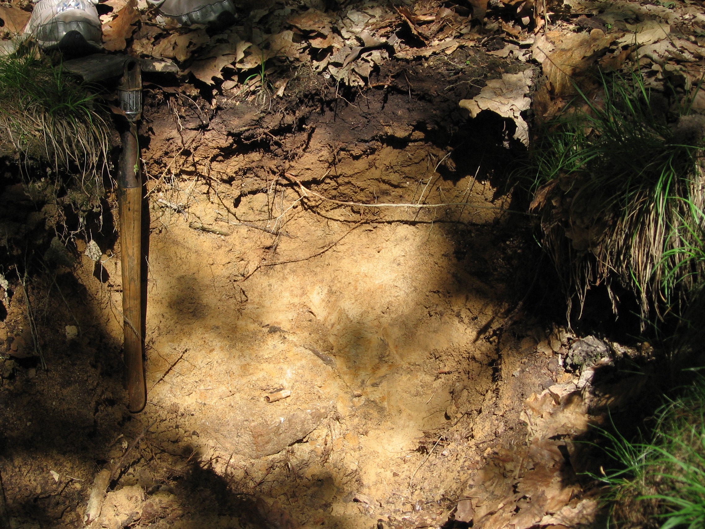
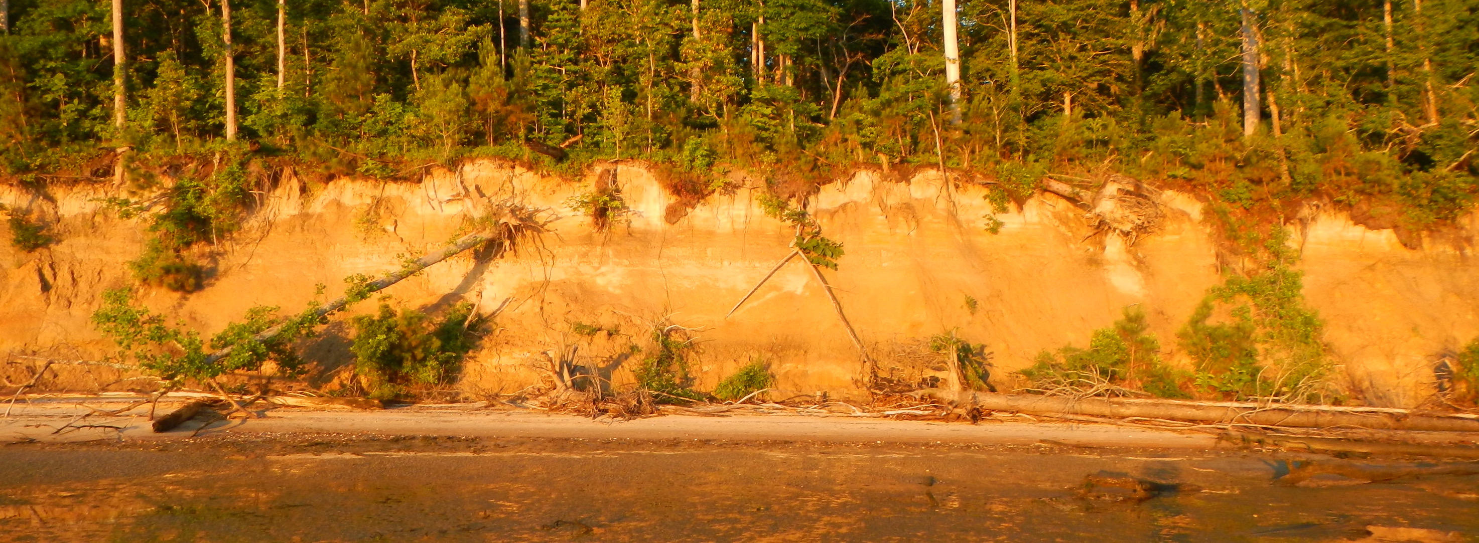
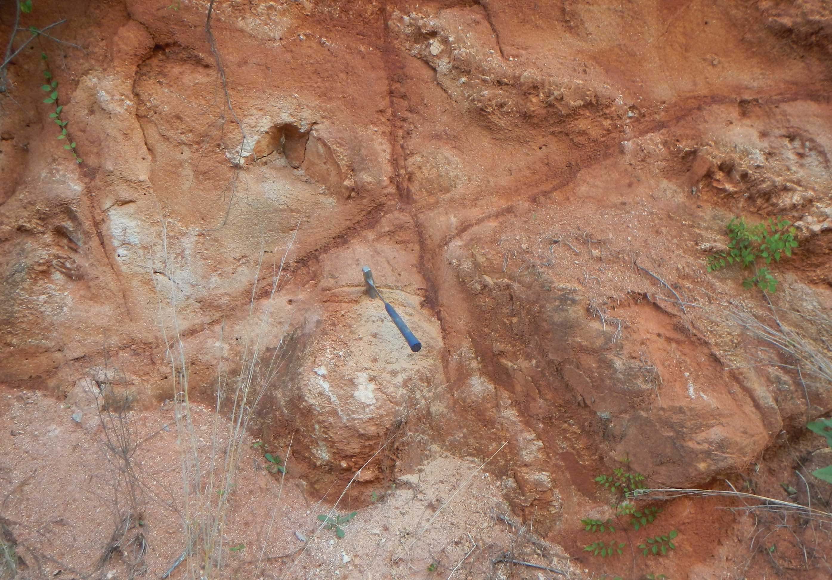
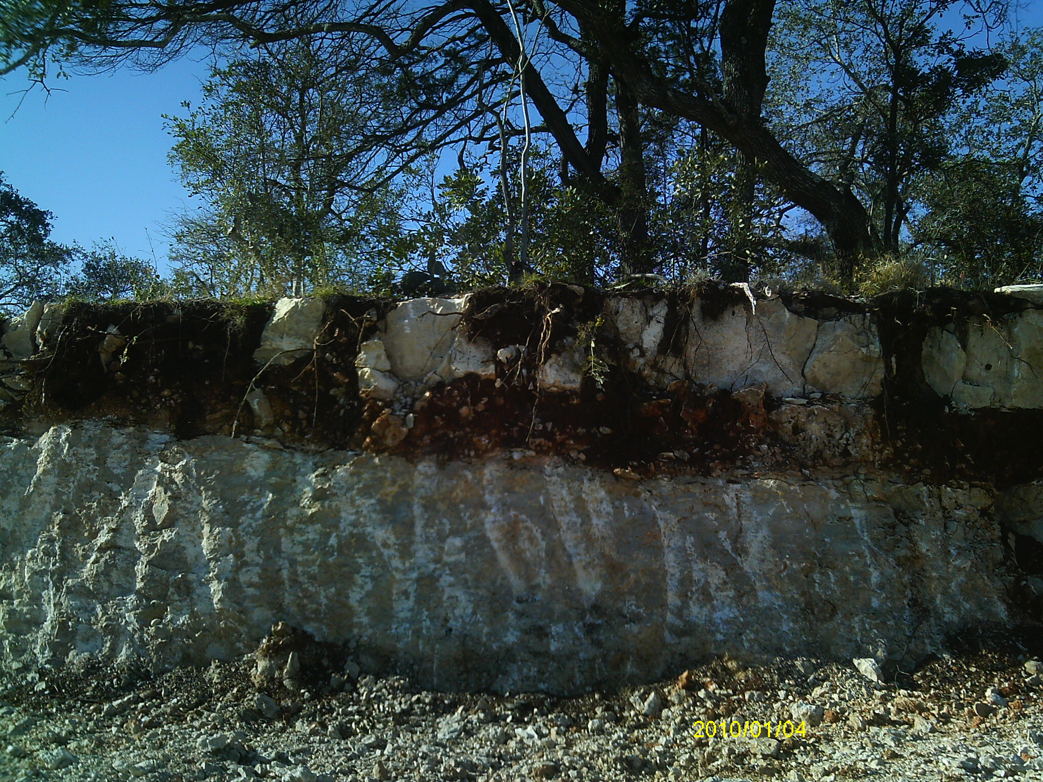
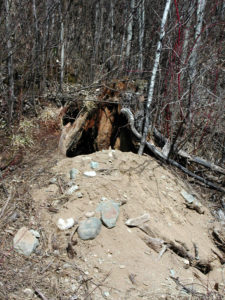
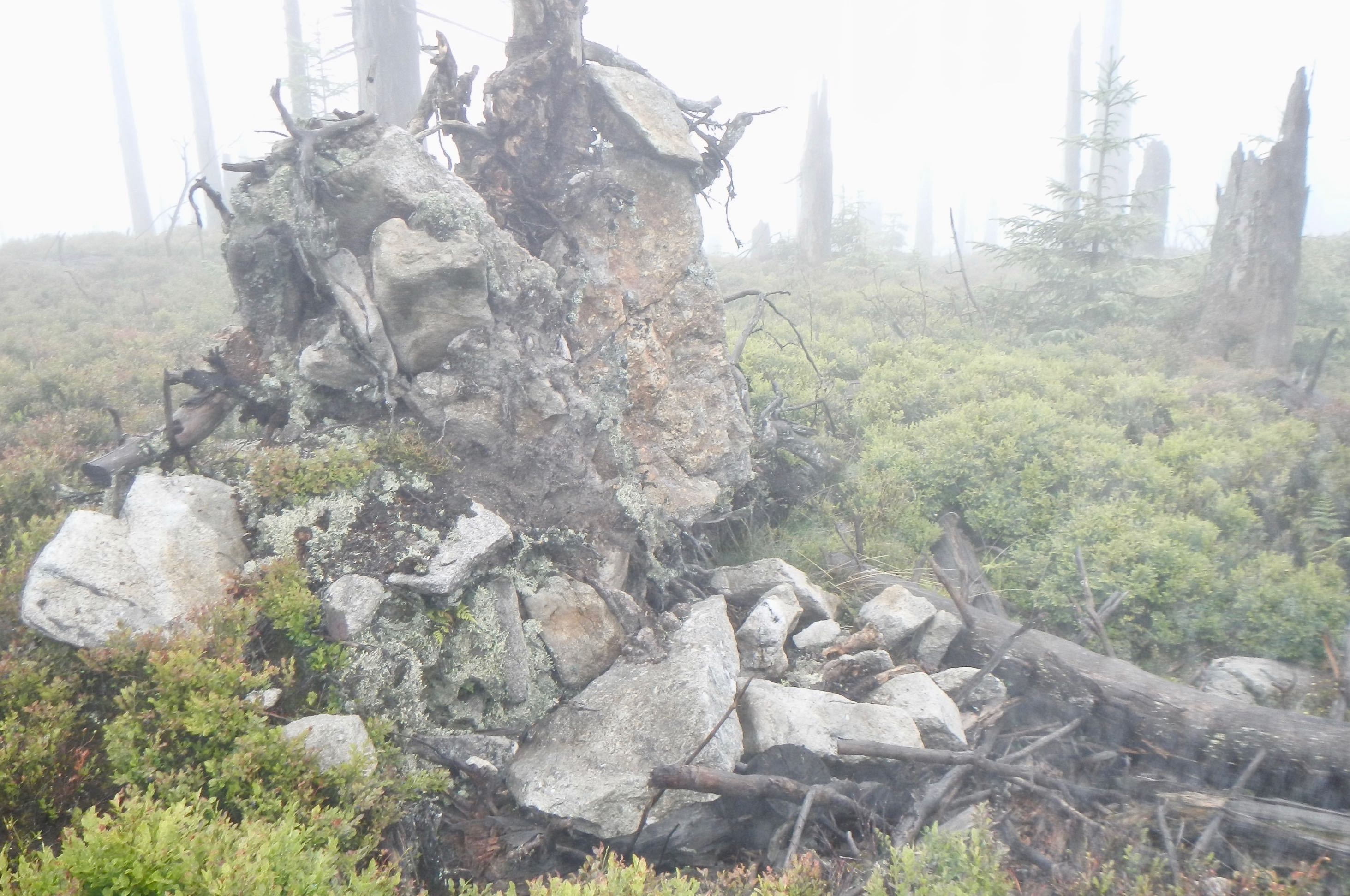
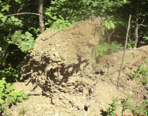
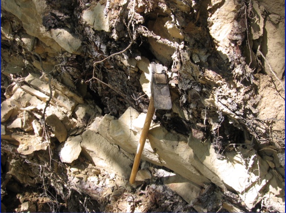
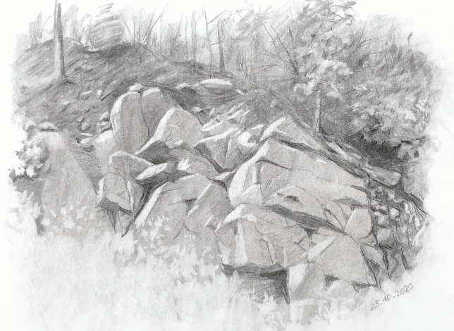
In the coastal plain, low relief, gentle slopes, and sandy soils with rapid infiltration had long been thought to be associated with very limited erosion. This impression was probably also promoted by visual comparison with the adjacent piedmont,  where exposed subsoils (red clay is an iconic symbol of the southern piedmont) and extensive gullies were common. By this point, the evidence from the river systems called this conventional wisdom into question. So I (and others) began to focus on erosion within the coastal plain. The bottom line is that coastal plain erosion rates are significant, and sometimes in the same ballpark as historical piedmont erosion rates (Phillips, 1993; 1997; Phillips et al., 1993; 1999a;b; Slattery et al., 1998). Again, I am only mentioning work I was involved in—others were coming up with similar findings.

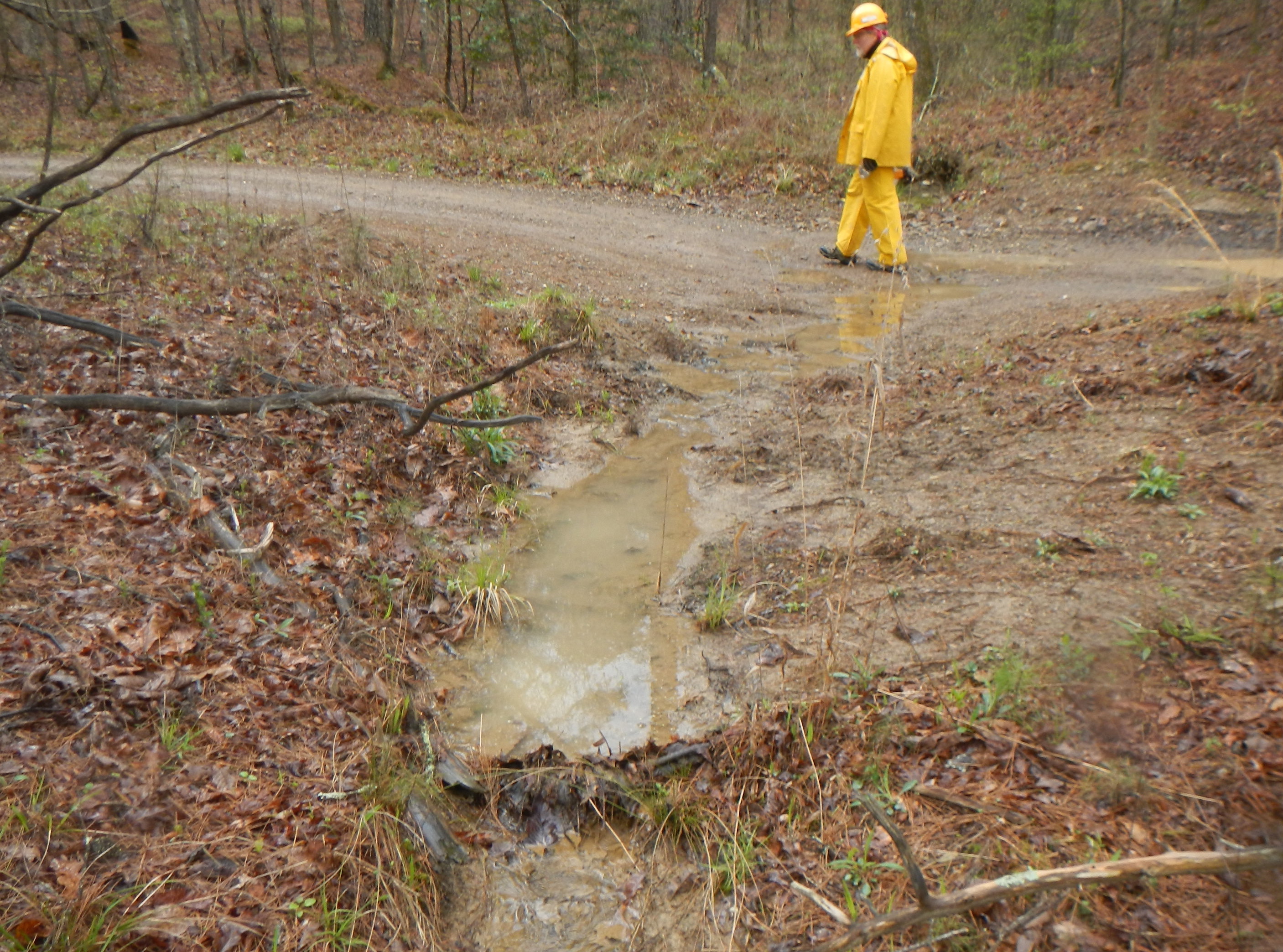
Why? The region also includes clayey soils that readily produce overland flow. And even in the sandy soils, high water tables promote saturation-excess runoff. On agricultural (and some silvicultural) land, artificial drainage systems are specifically designed to prevent ponding and keep surface runoff moving. Further, when runoff does occur the sandy topsoils are readily eroded and the clayey ones often include high contents of kandic clays that are easily dispersed in water (Phillips, 1997; Slattery et al., 1998; Slattery et al., 2006).

*  *  *  *  *

In the early 2000s, along with Mike Slattery of Texas Christian University and some of our students, I turned my attention to rivers of the Gulf of Mexico coastal plain in Texas (big shoutout to Greg Malstaff, then with the Texas Water Development Board who was vital in supporting this work). There the rivers feature some very large dams and reservoirs, and the coast has experienced extensive erosion. Many assumed—logically enough, given what was known at the time—a connection between sediment trapping by dams, reduced sediment supply downstream, and coastal erosion.

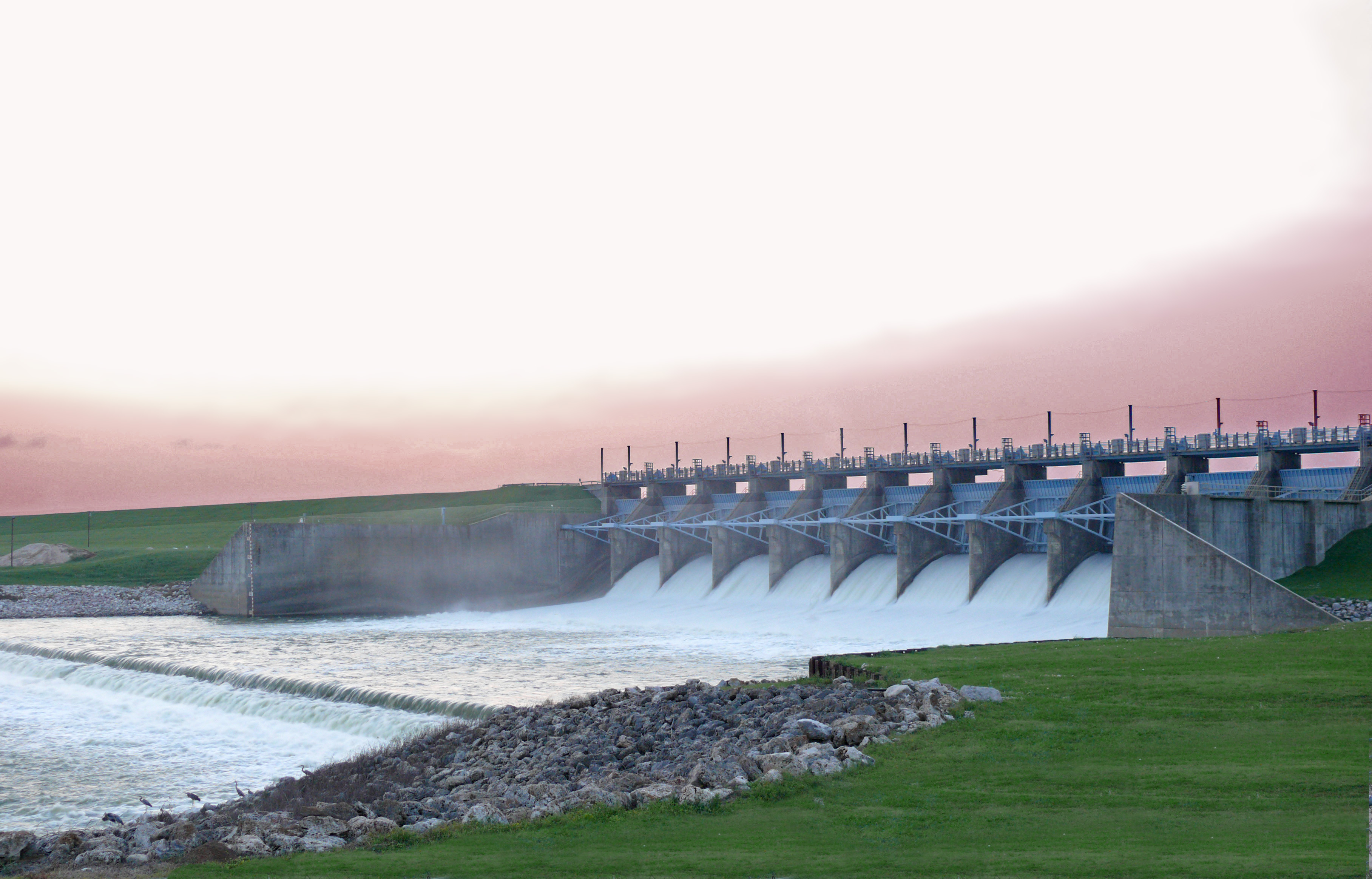
Livingston Dam

Working first on the effects of Lake Livingston and Livingston dam on sediments of the Trinity River, I confirmed that sediment yields at gaging stations upstream of the lakeand downstream indicate extensive sediment trapping in the lake and a major decline in sediment loads after dam construction. However, the Texas Water Development Board (TWDB) had also collected sediment data further downstream, at the upper end of the fluvial-estuarine transition zone, both before and after dam construction. These data showed NO post-dam reduction and extremely low sediment loads in both periods, suggesting that even before the dam was constructed not much fluvial sediment was making it to the lower river. The TWBD also has a nice database of repeated surveys of small and large lakes throughout the state. Those of the southeast Texas coastal plain showed quite significant sediment produced within the region. I first presented these data in Phillips and Musselman (2003), and in Phillips (2003a), in the context of arguing that long-term sediment yields may change little even when upstream erosion and sediment production changes dramatically.  In Phillips et al. (2004) we developed a more detailed sediment budget for the Trinity downstream of the dam. Sediment trapped in the lake is partially offset by channel erosion downstream of the dam (a common phenomenon often referred to as “hungry water”), and by the aforementioned erosion and tributary inputs from coastal plain sources. However, we also found that the lower river is a sediment bottleneck, with storage so extensive that upper and lower basins were essentially decoupled even before the dam. Dam-related sediment starvation effects occur for only 50-60 km downstream.

Though I did not directly examine sediment transport in the Sabine River, found consistent evidence that geomorphic impacts of the large Toledo Bend dam and reservoir were mainly confined to a relatively short zone downstream of the dam, and that effects of sediment trapping and flow regulation were nearly invisible in the lowermost river (Phillips, 2003b; 2008).

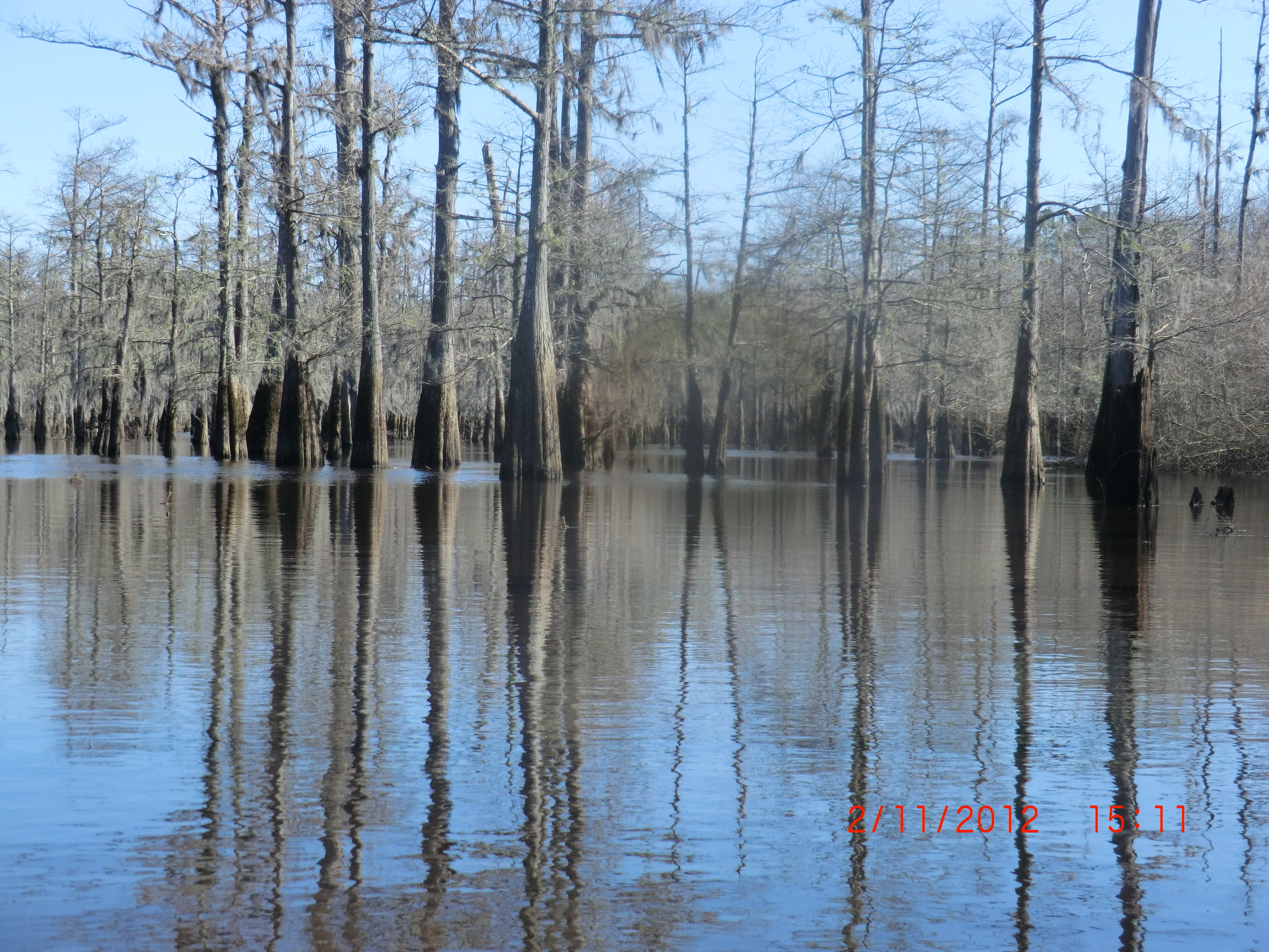
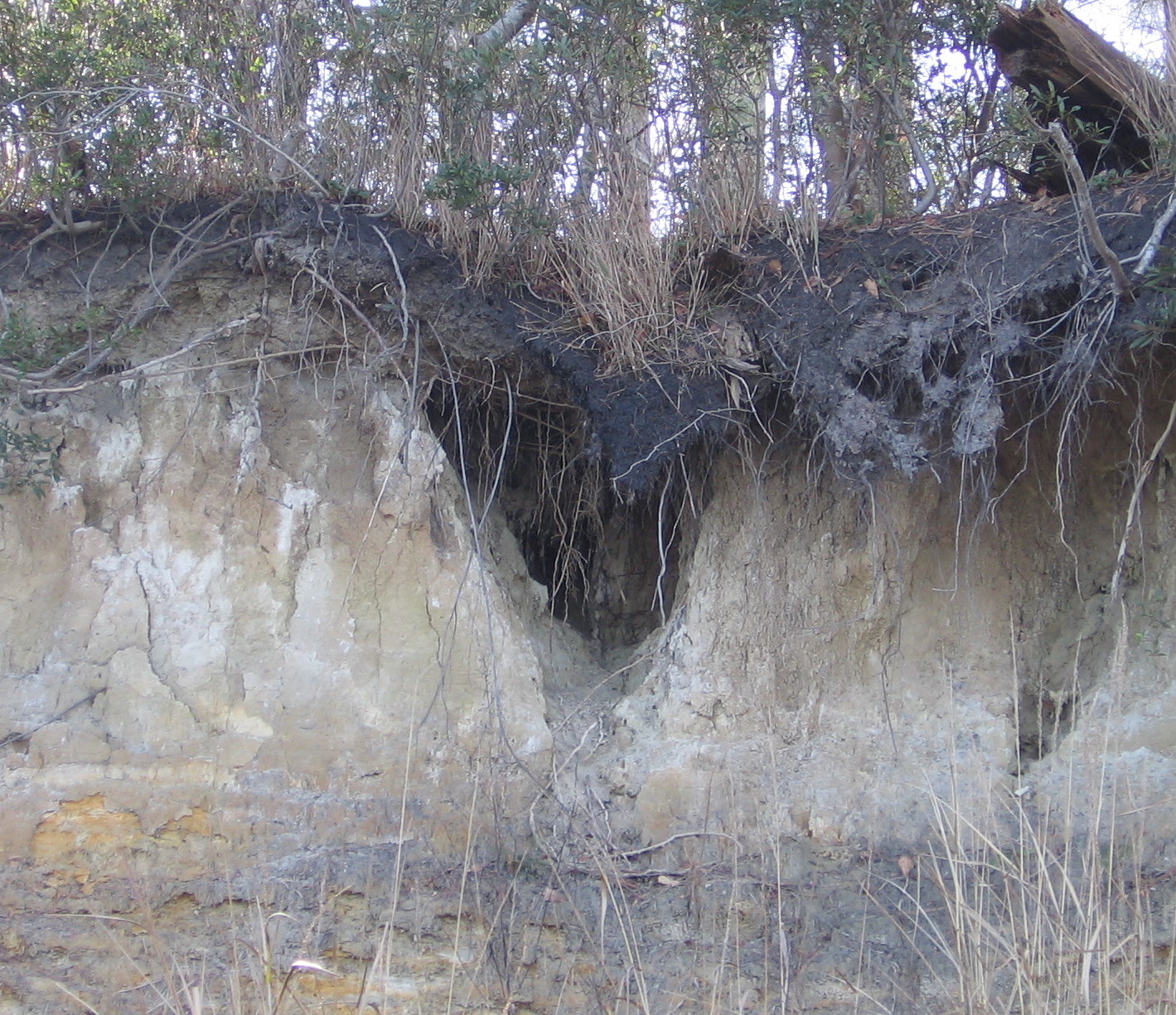
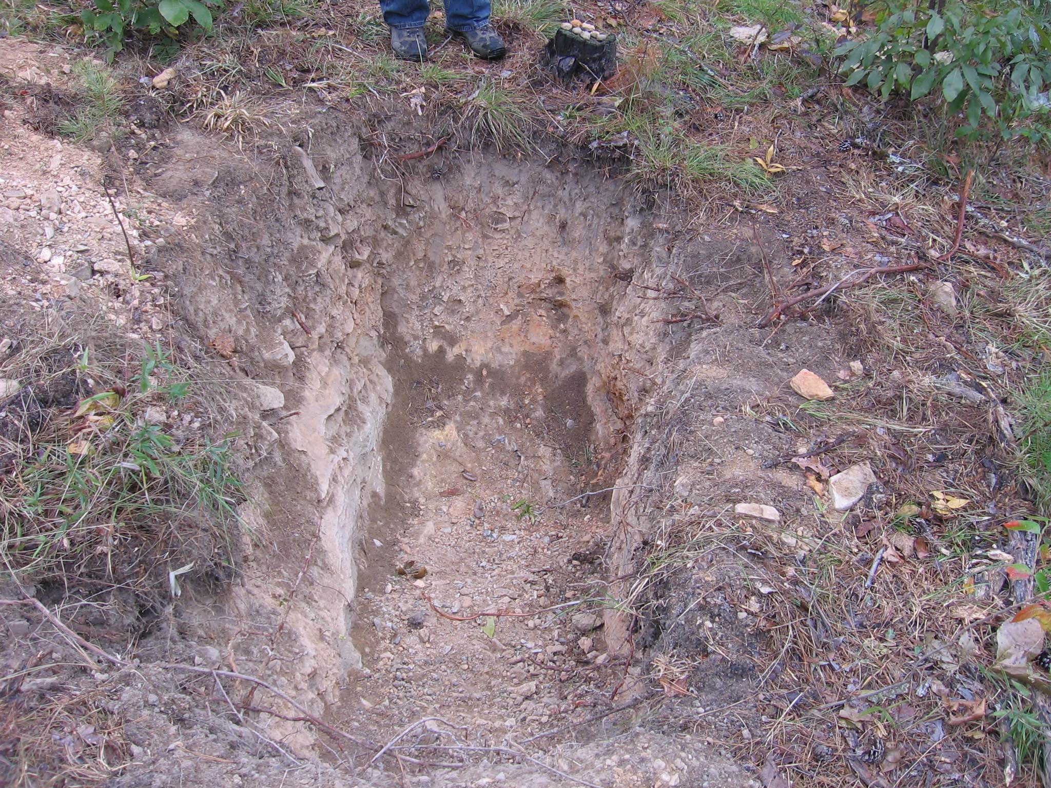
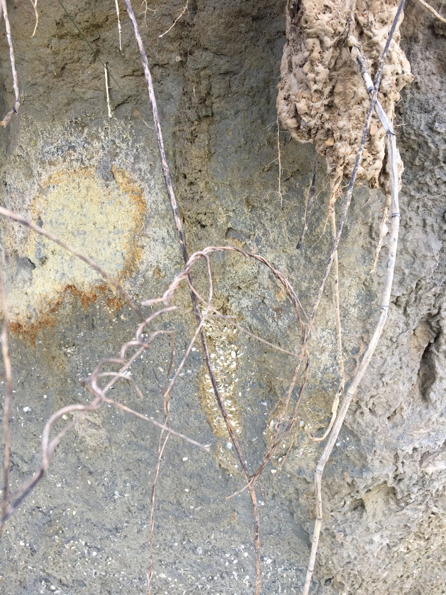
Floodplain depression on the lower Neches River, Texas.

A deeper dive into the lower Trinity showed that the extensive accommodation space in the lower River is strongly linked to antecedent Pleistocene morphology. The latter also results in sediment delivery to floodplain depressions during high flows, and the temporary conversion of tributaries to distributaries. Further, we documented low transport capacity in the lower river, and the absence of expected/presumed downstream trends in discharge, slow, and stream power (Phillips and Slattery, 2007).  We also examined sedimentation rates in the Trinity River delta, finding that modern fluvial sediment input is insufficient to account for Holocene sedimentation rates, implying non-fluvial sources in addition to river sediment (Slattery et al., 2010).

Based on our Texas and North Carolina experiences, Mike and I wrote a general overview of sediment storage and sediment delivery to the coast by coastal plain rivers (Phillips and Slattery, 2006; updated in Slattery and Phillips, 2010). A key idea is that in many cases the downstream-most gaging stations on most U.S. coastal plain rivers are a considerable distance from the estuaries, and well upstream of sediment bottlenecks in the fluvial-estuarine transition zones. Thus sediment data from these stations—whether they reflect increased loads from land use change or decreased loads from dams—do not reflect actual transport to the river mouth. We also highlighted the extensive storage bottlenecks in lower river reaches, storage in deltas and estuaries, and coastal backwater effects that extend well upstream of the estuaries.

*  *  *  *  *

Back to Rodriguez et al., 2020.

Their results indicate that these coastal depocenters have sediment sources other than fluvial watersheds upstream of dams, and that at least some of these inputs have increased since 1950.

    (Rodriguez et al., 2020).

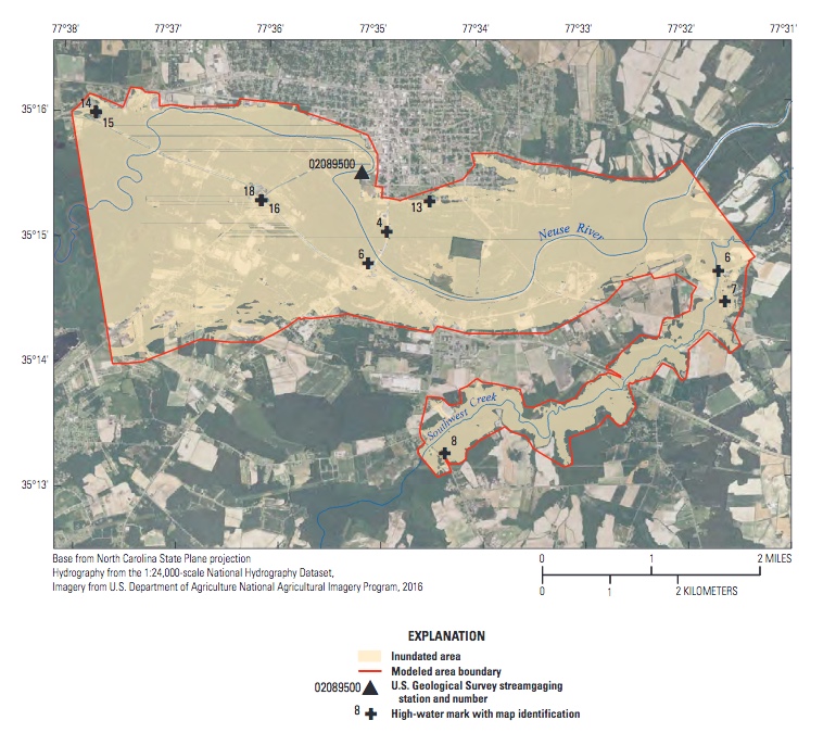
These sediment sources could include onshore transport of marine and coastal sediments and shoreline erosion in estuarine sites (this is, for example, the case in the North Carolina sites, nos. 6-8 in the figure above, and probably others).  Longshore transport along ocean and estuarine beaches, and resuspension and redistribution are also sources in some specific locations. Some of the depocenters in the study, such as Sabine Lake and Atchafalaya Bay, have been disturbed by human activities within the estuary, as well.

But Rodriguez et al. attribute the increase mainly to increased erosion and sediment production downstream of dams and lowermost gaging stations, and present evidence of population growth in these areas to support this. I agree—our studies in the North Carolina and Texas coastal plains show plenty of erosion to account for the increases.

*  *  *  *  *

Caveats and apologies: Again, the point of this was to highlight these new results and to review (reminisce?) about some of my own related work. Yes, I do feel like these new results support my past work. And yes, I do feel somewhat vindicated with respect to what we were finding in the 1990s and early 2000s. But I do not claim that we were the only ones discovering similar things, or that our work was not both inspired and informed by the studies of others.

References

Phillips, J.D. 1991a. Fluvial sediment budgets in the North Carolina Piedmont. Geomorphology 4: 231-241.

Phillips, J.D. 1991b. Fluvial sediment delivery to a Coastal Plain estuary in the Atlantic Drainage of the United States. Marine Geology 98: 121-134.

Phillips, J.D. 1991c. Upstream pollution sources and coastal water quality protection in North Carolina. Coastal Management 19: 439-449.

Phillips, J.D. 1992a. Delivery of upper-basin sediment to the lower Neuse River, North Carolina, U.S.A. Earth Surface Processes and Landforms 17: 699-709.

Phillips, J.D. 1992b. The source of alluvium in large rivers of the lower Coastal Plain of North Carolina. Catena 19: 59-75.

Phillips, J.D. 1993. Pre- and post-colonial sediment sources and storage in the lower Neuse River basin, North Carolina. Physical Geography 14: 272-284.

Phillips, J.D. 1997. A short history of a flat place: Three centuries of geomorphic change in the Croatan. Annals of the Association of American Geographers 87: 197-216.

Phillips, J.D. 2003a. Alluvial storage and the long term stability of sediment yields. Basin Research 15: 153-163.

Phillips, J.D. 2003b. Toledo Bend Reservoir and geomorphic response in the lower Sabine River. River Research and Applications 19: 137-159.

Phillips, J.D. 2008. Geomorphic controls and transition zones in the lower Sabine River. Hydrological Processes 22: 2424-2437.

Phillips, J.D., Golden, H., et al. 1999. Soil redistribution and pedologic transformations on coastal plain croplands. Earth Surface Processes and Landforms 24: 23-39.

Phillips, J.D., Musselman, Z.A. 2003. The effect of dams on fluvial sediment delivery to the Texas coast. Coastal Sediments ‘03. Proceedings of the 5th International Symposium on Coastal Engineering and Science of Coastal Sediment Processes, Clearwater Beach, Florida, p. 1-14.

Phillips, J.D., Slattery, M.C. 2006. Sediment storage, sea level, and sediment delivery to the ocean by coastal plain rivers. Progress in Physical Geography 30: 513-530.

Phillips, J.D., Slattery, M.C., 2007. Downstream trends in discharge, slope, and stream power in a coastal plain river. Journal of Hydrology 334: 290-303.

Phillips, J.D., Slattery, M.C., Gares, P.A. 1999. Truncation and accretion of soil profiles on coastal plain croplands: Implications for sediment redistribution. Geomorphology 28: 119-140.

Phillips, J.D., Slattery, M.C., Musselman, Z.A. 2004. Dam-to-delta sediment inputs and storage in the lower Trinity River, Texas. Geomorphology 62: 17-34.

Phillips, J.D., Wyrick, M., et al. 1993. Accelerated erosion on the North Carolina Coastal Plain. Physical Geography 14:114-130.

Rodriguez, A.B., McKee, B.A., et al. 2020. Coastal sedimentation across North America doubled in the 20th century despite river dams. Nature Communications 11, 3249; doi.org/10.1038/s41467-020-16994-z |

Slattery, M.C., Gares, P.A. et al. 1998. Quantifying soil erosion and sediment delivery on North Carolina coastal plain croplands. Conservation Voices 1(2): 20-25.

Slattery, M.C., Gares, P.A., Phillips, J.D. 2006. Multiple modes of runoff generation in a North Carolina coastal plain watershed. Hydrological Processes 20: 2953-2969.

Slattery, M.C., Phillips, J.D. 2010. Controls on sediment delivery in coastal plain rivers. Journal of Environmental Management 92: 284-289.

Slattery, M.C., Todd, L.M., et al. 2010. Holocene sediment accretion in the Trinity River delta, Texas, in relation to modern fluvial input. Journal of Soils & Sediments 10: 640-651.

Posted 17 December 2020