
geoscience

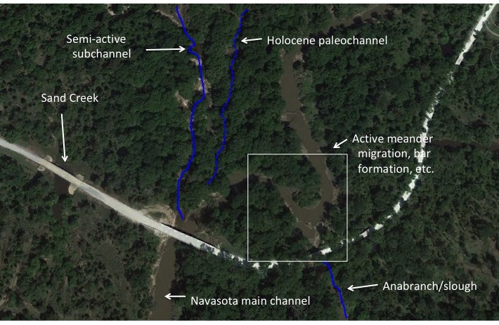
EVOLUTION OF DOLINE DIVERSITY

This post continues a series exploring the idea of evolutionary creativity in Earth Surface systems (ESS). Previous posts introduce the evolutionary creativityconcept, explore the possibility of algorithmic evolution modelsof ESS, and discuss the appearance over time of new varieties of landforms

-------------------------------------------------------------------------------------------------------

Biologists have put a great deal of effort into identifying the variety of life forms. While there is only one extant species of the genus Homoand 11 of Canis, there are more than 600 species of Quercus (oak trees) and >350,000 of beetles (and counting).  

THE APPEARANCE OF NEW VARIETIES OF LANDFORMS

This continues a discussion that started by considering the possibility of evolutionary creativity in landscapes and continued by exploring the possibility of algorithmic evolution models of Earth surface systems (ESS). 

In biological evolution by natural selection, new varieties arise via genetic mutations. Occasionally one of these turns out to be advantageous--the fitness of the organism is increased, and the variation is "selected" (recall that Darwin used natural selection to contrast with selective breeding of animals and plants by humans). The selected organism can reproduce, and pass the selected trait to its progeny.

ALGORITHMIC EVOLUTION MODELS OF EARTH SURFACE SYSTEMS?

This post is a continuation of a thread that starts here.

The algorithmic evolution models pioneered by Gregory Chaitin (see Proving Darwin,2012 for a very readable introduction) are based on a metaphor of an organism as a K-bit program that takes the original organism and produces a mutated organism A'. The fitness of the organism/algorithm is measured by the largest integer the algorithm can calculate. Thus a mutation that increases the largest calculable number is retained, while others are rejected. This continues until BB(N), defined as the largest integer that can be produced by a <N-bit program that produces a single integer and then halts. 

This is a plausible analog for biological evolution, in which continuous improvement in fitness is possible, up to some maximum limit. In nature the maximum limits are presumably associated with maximum rates of biological processes rather than algorithmic complexity and information (i.e., BB(N), which has the awesome name of the Busy Beaver Number). 

HOTSPOTS OF LATERAL CHANNEL CHANGE

Recently I had the pleasure of visiting the geography department at Texas A&M, and during my trip I was able to revisit some field sites along the Navasota River I had last been to in 2006. The lower Navasota is basically an anastamosing system--there is a single dominant channel, but multiple subchannels, some active at normal and low flows, at any given valley cross-section. One place is particular, Democrat Crossing, is a particularly confusing locus of recent and ongoing channel change. 

2017 Google EarthTMimage of Democrat Crossing. Sand Creek is actually a perennial or active Navasota River subchannel (semi-active means, in my lingo, that it usually carries flow, but may dry up in low-flow periods). Some of the subchannels have been highlighted with blue lines I added, as you can't really see them if you don't already know they are there. 

EVOLUTIONARY CREATIVITY IN LANDSCAPES?

More than one scholarly observer has remarked in the contrast between physics, characterized mostly by deterministic, hard-and-fast laws that operate the same way everywhere and always (at least the Newtonian physics that apply to Earth sciences) and biology. Biology is portrayed as being much more fluid and dynamic, in the sense that chance (e.g., mutations) and environmental adaptations play a major role. As Gregory Chaitin (2012; a mathematician, by the way, not a biologist) puts it, biota and evolution are creative, while physics is not. This tension is sometimes portrayed or exemplified as a Newtonian (as in Isaac Newton) vs. Darwinian (i.e., Charles Darwinian) outlook. 

I have much love for both Newton (left) and Darwin, but have chosen to follow Darwin with respect to my hairstyle. 

FLUVIOKARST CHRONOSEQUENCES

Historical contingency in fluviokarst landscape evolution was just published in Geomorphology 303: 41-52.  When I first came to central Kentucky in 2000 I began noticing the strong contrasts in landscape and landform development on inner vs. outer Kentucky River incised meander bends. Investigating this and related phenomena has occupied me off and on ever since. Only a few years ago I realized that given the nature of bend development over the past 1.5 Ma or so, the bend interiors represent a chronosequence of landforms. This paper exploits those chronosequences, using graph theory, to explore the role of historical contingency.


Chronosequence of strath terraces (T1, T2, T3) and other geomorphic surfaces at Polly’s Bend, Kentucky. The surfaces nearest the river are youngest; those farther away are oldest.

DOES RAINDROP SIZE MATTER?

Below is a picture of raindrop impact craters after a rain last month on a beach along the Neuse River estuary, N.C. The spot pictured has no overhanging trees or anything else, so the craters represent direct raindrop impacts. As you can see, assuming crater size is related to drop size, they represent a large range (the largest craters pictured are roughly 10 cm in diameter; the craters must be at least slightly larger than the drops). Rainsplash is a significant factor in soil erosion--even if not directly important, the process is key for dislodging grains or particles that are then transported by runoff. Drop impact also influences surface crusting and sealing, and thereby hydrological response. So, I got to thinking, what is the potential significance of such a large variation in drop size?

Kinetic energy is given by KE = 0.5 m V^2, where m is mass in kg, and V is velocity in m/sec. A 2 mm diameter raindrop has a mass of 4.19 mg and a terminal velocity of about 6.26 m/sec. This gives a kinetic energy of about  0.00008 joules per raindrop.

BIRTH OF FERRICRETES

Ferricretes are soil or sediments cemented together by iron oxides. In eastern North Carolina, reducing conditions often prevail on the broad, flat interfluves. Under these conditions Fe is reduced, and soluble. Groundwater flow from these areas toward the major river valleys transports this dissolved ferric iron. When the groundwater discharges along the valley side slope it comes in contact with oxygen, and the iron oxidizes to its ferrous form. These iron oxides coat whatever material exists at that location--sand, clay, etc.

Limonite ferricrete at Fishers Landing, NC. The piece at the top is about 40 cm long. 

PATH EXTINCTION & REINFORCEMENT

The development and change over time (evolution) of geomorphic, soil, hydrological, and ecosystems (Earth surface systems; ESS) is often, perhaps mostly, characterized by multiple potential developmental trajectories. That is, rather than an inevitable monotonic progression toward a single stable state or climax or mature form, often there exist multiple stable states or potentially unstable outcomes, and multiple possible developmental pathways. Until late in the 20th century, basic tenets of geosciences, ecology, and pedology emphasized single-path, single-outcome conceptual models such as classical vegetation succession; development of mature, climax, or zonal soils; or attainment of steady-state or some other form of stable equilibrium. As evidence accumulated of ESS evolution with, e.g., nonequilibrium dynamics, alternative stable states, divergent evolution, and path dependency, the "headline" was the existence of > 2 potential pathways, contesting and contrasting with the single-path frameworks. Now it is appropriate to address the question of why the number of actually observed pathways is relatively small.The purpose of this post is to explore why some developmental sequences are rare vs. common; why some are non-recurring (path extinction), and some are reinforced.

Subscribe to geoscience